Augmented Half-Life Estimation Based on High-Frequency Data
Abstract
Half-life estimation has been widely used to evaluate the speed of mean reversion for various economic and financial variables. However, half-life estimation for the same variable are often different due to the length of the annual time series data used in alternative studies. To solve this issue, this paper extends the ARMA model and derives the half-life estimation formula for high-frequency monthly data. Our results indicate that half-life estimation using short-period monthly data is an effective approximation for that using long-period annual data. Furthermore, by applying high-frequency data, the required effective sample size can be reduced by at least 40% at the 95% confidence level. Copyright © 2015 John Wiley & Sons, Ltd.
Introduction
The early concept of half-life comes from the natural science field. Half-life is used to measure the amount of time it takes for half of a substance to decay. Until recently, the idea of a half-life has been widely applied for assessing the speed of mean reversion or persistence in economic and financial variables (e.g. exchange rate, interest rate, oil price and stock price) by economists. The main reason for this is that half-life gives the slowness of a mean reversion one observable time, and can even demonstrate a relationship with the business cycle. Unfortunately, the limited amount of data always causes difficulty in determining true half-life by adopting existing methodology. Therefore, this paper seeks to further improve the formula of half-life to tackle this issue.
In the past, several scholars discussed and suggested methods to measure half-life. For example, Aduaf and Jorion (1990) first built a half-life estimation formula based on the AR(1) process.1 Next, Stock (1991) employed an Augmented Dickey–Fuller (ADF) regression to estimate the confidence interval of half-life, after which Andrews (1993) adopted an AR(1) process to propose a measure of the half-life of a unit shock (HLS), which gives the length of time until the impulse response of a unit shock is half of its original magnitude (see Andrews, 1993, p153). Furthermore, Andrews and Chen (1994) substituted the AR(p) process for the traditional ADF regression form to obtain the coefficients of an approximate median unbiased estimate. However, two shortcomings still exist in the traditional half-life formula based on AR(1), and these need to be resolved. One is limited data length and the other is missing lag length. Therefore, how to measure half-life is still a continual concern (e.g. Taylor, 2001; Mark, 2001; Rossi, 2005; Chambers, 2005; Seong et al., 2006).
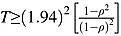
In terms of data length, until now most scholars have only used annual data based on an AR(1) model to estimate half-life and its confidence interval. When the series is a slow mean reversion process, long annual data are usually needed to estimate half-life. This observation is also shown in Table 1. According to the HLS, which was built by Andrews (1993), when a half-life is 13.53 years then at least 147 years of annual data are needed to estimate it (based on a 95% confidence level).2 In fact, there is usually a lack of sufficiently long annual samples to measure it, especially in terms of some commodity price data. To resolve the sample size, recent large papers have begun to use high-frequency data (e.g. daily, weekly and monthly data) to replace annual data to discuss the price behavior. However, an interesting question arises: can half-life based on annual data be estimated by high-frequency data? Luckily, the answer seems to be explained by Taylor (2001) and Chambers (2005). Above all, Taylor (2001) considers that although, in practice, data cannot always be directly observed, the average value of data over all time is available for observation. Accordingly, based on the condition that the annual data and high-frequency data are both the AR(1) model, Taylor developed a new methodology which uses high-frequency data transfer to annual data to estimate half-life. Under the same assumptions, Chambers (2005) also derived the same formula. According to the implications of the methodological innovations of Taylor (2001) and Chambers (2005), the coefficients (parameter β) of high-frequency data derived from the coefficients (parameter β) of annual data can be used to estimate long-run half-life. However, in their derivative formula, they ignore the probability that high-frequency data can produce high lag length. As Seong et al. (2006) state, when an AR(1) process at a higher frequency is aggregated and observed at a lower frequency, this observed process should become an ARMA(1, 1) process (see Seong et al., 2006, p.2058).
| ρ | T | H |
|---|---|---|
| (yearly) | (year) | (half-life) |
| 0.95 | 146.78 | 13.51 |
| 0.90 | 71.51 | 6.58 |
| 0.85 | 46.42 | 4.27 |
| 0.84 | 43.28 | 3.98 |
| 0.83 | 40.51 | 3.72 |
| 0.82 | 38.05 | 3.49 |
| 0.81 | 35.85 | 3.29 |
| 0.80 | 33.87 | 3.11 |
| 0.79 | 32.08 | 2.94 |
| 0.78 | 30.45 | 2.79 |
| 0.77 | 28.96 | 2.65 |
| 0.76 | 27.60 | 2.53 |
| 0.75 | 26.35 | 2.41 |
| 0.74 | 25.19 | 2.30 |
| 0.73 | 24.11 | 2.20 |
| 0.72 | 23.12 | 2.11 |
| 0.71 | 22.19 | 2.02 |
| 0.70 | 21.33 | 1.94 |
In terms of the lag length, compared to Taylor (2001) and Chambers (2005) an in-depth study by Mark (2001) and Rossi (2005) further proposed a measure of half-life for a general AR(p) model and its confidence intervals, respectively. In addition, Seong et al. (2006) also extended the AR(1) to ARMA(1, 1). Even if they add more lag length or one moving average in their non-AR(1) model to estimate half-life, different from Taylor (2001) and Chambers (2005), their formula cannot resolve the difference of the coefficient (parameter ρ), especially when using high-frequency data transfer to annual data, since it is easy for the aggregate process to produce a biased estimation.
More concretely, 100 years’ sunspots series from 1850 to 1950 can be taken as an example to explain why the existing half-life formula cannot capture true half-life, especially in high-frequency data. According to NASA's calculation, the average length of a sunspot cycle (SSC) is around 11 years (sometimes the sunspot cycle can be as short as 9 years and other times as long as 14 years, but on average it takes 11 years). That is, the true half-life of sunspots is an average 2.75 years in the long run (its range is from 2.25 years to 3.5 years). The result can be observed using a regular sunspot cycle chart (see Figure 1: there are nine cycles in 100 years’ sunspots data). Similarly, a so-called ‘half-life’ formula can also be adopted to estimate it. According to the AR(1) formula, the half-life of annual data is 3.18 years but for monthly data it is about 0.61 years. Clearly, the half-life of the annual data (3.18 years) falls somewhere within the interval of the true half-life of sunspots (2.25 to 3.5 years), but differs significantly from the half-life based on high-frequency data (0.61 years). Accordingly, Taylor (2001) and Chambers (2005) methodology and Seong et al.’s (2006) formula are adopted to re-estimate the half-life of the monthly data to be 1.01 years and 0.58 years, respectively. Unfortunately, compared with the annual result (3.18 years), their estimators still cause significant bias (see Table 2). In other words, the existing formula cannot capture the true half-life, especially in high-frequency data. In statistics, the bias of the estimator can come from the missing lag length (e.g. the estimated model) as well as from the difference in coefficients (e.g. the estimated parameters). Therefore, it seems to be necessary to extend the ARMA model based on Taylor (2001) and Chambers (2005) methodology to reduce the errors.

In order to achieve this aim, a Yule–Walker equation is first applied to extend the formula of half-life based on the high-frequency ARMA model of Seong et al. (2006), and then Taylor (2001) and Chambers (2005) methodology is adopted to modify the coefficients of the annual AR(1) model. Next, this paper uses 100 years’ stationary sunspots data from 1850 to 1950 to estimate the half-life by means of a new formula based on modifying the ARMA model: equation 17. Finally, the numerical results provide two main findings, the first of which is that it is feasible to use short and high-frequency data to replace long and low-frequency data to estimate slow half-life, and this can indeed obtain approximate results of true half-life. Secondly, at a 95% confidence level, the new innovation can save around at least 40% of samples and, furthermore, it can be applied to future research in different fields.
The remainder of this paper is organized as follows: the next section discusses half-life and the ARMA model, the third section presents the numerical results and the final section concludes.
Half-Life and the ARMA Model
 (1)
(1) (2)
(2) (3)
(3) (4)
(4) is the asymptotically median-unbiased (AMU) estimator of ρ, cmed is determined using Stock's (1991) Table A-1 and
 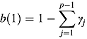 .
. (5)
(5) (6)
(6) . Meanwhile,
  is also shown in Box et al. (1994, p. 81); Maddala and Kim (1998, p. 17) and Enders (1995, p. 81).
 (7)
(7) (8)
(8)This is shown in Appendix A.
 (9)
(9) (10)
(10) (11)
(11) (12)
(12) , β = ρ1.
 (13)
(13) (14)
(14)
All proofs are provided in Appendix B.
 (15)
(15) (16)
(16) (17)
(17)Numerical Results
To prove whether equation 17 can exactly capture the true half-life in the long run or not, natural science data are adopted in the form of sunspots covering the period from 1850 to 1950, for which the data are obtained from the National Geophysical Data Center (NGDC) to support our idea. First, the ADF unit root test is used with the intercept (see Figure 1) to assess whether or not the sunspots are unit roots, and the results show that the sunspots are robust stationary series (see Table 3).
| Sample type | Period | Lag length | ADF (intercept) | |
|---|---|---|---|---|
| Level | First difference | |||
| Yearly data | 1850–1950 | 2 | −8.2197*** | −8.6022*** |
| Monthly data | 1850:m1–1950:m12 | 3 | −4.0986*** | −21.3884*** |
- Note: The null hypothesis of ADF is H0: variable has a unit root and test critical value is from MacKinnon (1996). (2) Asterisks indicate significance at
- *** 1%.
Next, the plan is to use different sample sizes to estimate the half-life of stationary sunspots. As already mentioned, in fact, a 3.18-year half-life of sunspots which is estimated by 100 years’ annual data is sufficient to represent the true half-life of the sunspots. Accordingly, as shown by the calculations in Table 1 (based on a 95% confidence level), it can first be calculated that a half-life of 3.18 years needs at least 35 years’ annual data. That is, the half-life of annual data is measured in samples which are larger than 35 years. Then, they are divided into 17 groups (every 50, 45, 40, 35, 30, 25, 24, 23, 22, 21, 20, 15, 14, 13, 12 years) to estimate the half-life of the monthly data.
These results are presented in Table 4. The remainder is all results of monthly data, except for column 2 of Table 4, which is yearly data. It can be seen from columns 3–5 of Table 4 that, no matter which formula developed by Taylor (2001); Chambers (2005) or Seong et al. (2006) is used to estimate the half-life, the results are far from the true half-life based on annual data (compared with 3.18 years in Table 2 and the results of the year's data in column 2 of Table 4). However, using high-frequency data based on equation 17 by the AICc rule,5 the true half-life in the long run can be exactly estimated (results in column 6 of Table 4 are 3.08–3.32 years). Hence, compared with annual data based on AR(1) monthly data based on the selected ARMA model by the AICc rule should be a suitable estimator for yearly data based on AR(1) in this case. The confidence intervals of all groups are marked and lines drawn (the black solid line is the mean value; the black dashed line represents a boundary) in Figure 2.
| Sample size | Average half-life (years) | ||||
|---|---|---|---|---|---|
| Yearly data AR(1) | Monthly data | ||||
| ARMA(1, 0) | ARMA(1, q) | ||||
| Equation 9 | Equation 17 | Equation 9 | Equation 17 | ||
| Every 50 years | 3.16 | 0.50 | 0.84 | 0.47 | 3.13 |
| Every 45 years | 3.10 | 0.49 | 0.83 | 0.47 | 3.11 |
| Every 40 years | 3.12 | 0.50 | 0.84 | 0.47 | 3.12 |
| Every 35 years | 3.04 | 0.50 | 0.85 | 0.47 | 3.08 |
| Every 30 years | — | 0.51 | 0.86 | 0.48 | 3.13 |
| Every 25 years | — | 0.51 | 0.87 | 0.49 | 3.16 |
| Every 24 years | — | 0.52 | 0.87 | 0.49 | 3.14 |
| Every 23 years | — | 0.52 | 0.87 | 0.49 | 3.17 |
| Every 22 years | — | 0.52 | 0.87 | 0.49 | 3.19 |
| Every 21 years | — | 0.52 | 0.87 | 0.50 | 3.22 |
| Every 20 years | — | 0.52 | 0.87 | 0.51 | 3.26 |
| Every 15 years | — | 0.51 | 0.85 | 0.49 | 3.29 |
| Every 14 years | — | 0.50 | 0.85 | 0.49 | 3.29 |
| Every 13 years | — | 0.51 | 0.85 | 0.49 | 3.28 |
| Every 12 years | — | 0.51 | 0.86 | 0.49 | 3.32 |
- Note: The ARMA(1, q) model is selected based on the AICc rule.

Furthermore, according to Figure 2, it can be found that half-life based on annual data (Tables 2 and 4—from 3.04 to 3.18 years) is all at a 95% confidence interval (CI) of half-life based on monthly data. That is, equation 17 can be used to estimate the true half-life exactly. Meanwhile, it should be considered that if a 3.18-year half-life needs 35 years then it can be clearly seen from Figure 2 (vertical black dot-dashed line) that 246–252 months’ data can also obtain an approximate half-life with a confidence interval still within the boundary of the true half-life of sunspots (black star line). In other word, it can save at least 170 months of samples (40% samples).
Accordingly, these numerical results not only robustly support the modified formula of half-life—equation 17, which adopts Taylor (2001) and Chambers (2005) methodology to modify the ARMA(1, q) and can reduce the limited data, especially when high-frequency data is used to estimate half-life—but also save samples.
In summary, in the case of sunspots, it can be considered that half-life based on the ARMA model should be reasonable when high-frequency data is adopted to replace annual data to estimate long-run half-life. That is, the modified half-life formula can also be widely used in related estimates in different fields.
Conclusions
A limited amount of data always causes difficulty in determining true half-life when using existing methodology. Although some existing papers provide new methodology to measure half-life, the bias of the estimator still exists, especially in high-frequency data. To improve these estimators, this paper provides a new measure methodology which is based on a high-frequency ARMA(1, q) model and selected by the AICc rule to capture the true half-life of an annual AR(1) model. According to the innovation, the results of half-life are modified based on high-frequency data. Our numerical results provide two main findings, the first of which suggests that half-life based on high-frequency data should adopt a new formula—equation 17—to measure the true half-life in the long-run. The results show a good estimator for annual data. Secondly, at a 95% confidence level, this innovation can save at least 40% of samples.
Furthermore, the innovation that is built on a high-frequency ARMA (1, q) model to estimate an annual AR (1) model can replace the traditional formula, which only uses annual data to estimate half-life. Above all, short and high-frequency data could be used to obtain a consistent half-life with long annual data.
 .
. (see Postali and Picchetti, 2006, p. 515; Maddala and Kim, 1998, p. 62).
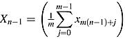
 is yearly data (s = 0, 1, …, S − 1), then
 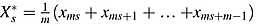 can be represented where m = 12 and
  .
.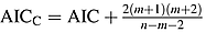 , where m = (p + q) and n is sample size. For example, if the model is ARMA(1, 2), then p = 1 and q = 2 (see Hurvich and Tsai, 1989, p. 300, equation 4).
Biographies
Mao-Lung Huang Assistant professor, Department of Hotel Management, Tainan University of Technology, Taiwan.
Shu-Yi Liao Associate Professor, Department of Applied Economics, National Chung Hsing University, Taiwan.
Kuo-Chin Lin Professor, Department of Business Administration, Tainan University of Technology, Taiwan.
References
Appendix A: ARMA(1, Q)
 ()
() ()
() ()
() ()
() ()
() ()
()Appendix B: ARMA(1, q) Based on High-Frequency Data Transfer to AR(1) Based on Annual Data
 ()
() ()
() ()
() ()
() ()
() ()
() and
and 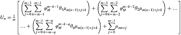
 ()
() ()
()
 ()
()

 ()
() ()
() ()
()


 ()
()