Testing a multimedia compartmental model with monitoring data
Abstract
Based on its geographic similarity and nested structure, a chemical transport and transformation model developed in The Netherlands was adopted to a nine-parish, 5,400-km2 area in southern Louisiana, USA, and tested for its ability to predict concentrations in the environment. SimpleBox 2.0 represents a class of models that compartmentalize the air, water, soil, sediment, and plants into boxes while maintaining a high degree of detail for processes within and between boxes. Past use has been in the evaluative mode, primarily where qualitative predictions of chemical behavior and distribution are made. Limited testing of model-predicted versus measured concentrations have been attempted. In recent years, quality and quantity of emission and monitoring data have improved dramatically. Such information was used in calibration and validation exercises with eight chemicals in the Louisiana chemical corridor, which receives inputs from urban, industrial, and agricultural sources. Geographically, the corridor was nested within the state of Louisiana, which was in turn nested within the continental United States. Parameter sensitivity studies, including transport coefficients, temperature, and degradation half-life revealed that the latter produces the largest range of variation in predicted concentrations. Published half-life data were used with benzene, vinyl chloride, 1,1,1-trichloethane, and atrazine in a calibration phase with 1995 monitoring data at steady state; this allowed selection of the appropriate emission database. A validation exercise was performed with toluene, styrene, trichloroethylene, and metribuzin. Predictions were compared to average measured concentrations. Atrazine and metribuzin reside primarily in the water; the others reside in the air. The predicted concentrations for benzene, metribuzin, and trichloroethylene were low by a factor of less than two. Vinylchloride, toluene, and 1,1,1-trichloroethane were low by factors between 3 and 10. Styrene and atrazine were low by factors of 45 and 65, respectively.
INTRODUCTION
Multimedia environmental models were introduced in the 1970s and have proven to be powerful tools that integrate information on emissions, chemical properties, environmental characteristics, and transport processes into a comprehensive framework for assessing the fate and distribution of chemicals entering the environment [1, 2]. These models are of simple structure and use the Lavoisier mass balance. Species mass balances that describe chemical movement and transformation within and between compartments give first-principle power to the final mathematical algorithm. The use of well-mixed compartments, referred to as boxes, representing the different environmental media (air, water, soil, sediment, and biota) is viewed as a major weakness. Simplicity alone is not necessarily a fatal flaw; however, misinterpretation and misrepresentation of results by the nonexpert user are problematic. Testing predictions against monitoring data provides one means of arriving at some understanding of the strengths and limitations of these models.
A nine-parish region along the Mississippi River between Baton Rouge and New Orleans, Louisiana, USA, termed the chemical corridor, has significant urban, industrial, and agricultural chemical sources. This, along with measured concentrations, make it a good choice for calibration and validation studies. The specific objectives of this study are to adapt a multimedia model to describe chemical behavior in the corridor; to use published emissions and other data to predict the concentrations within selected media; to use published monitoring data in calibration, validation, and uncertainty characterization exercises; and, based on the results, to draw conclusions about model testing and the ability of multimedia environmental models to make real-world predictions of chemical concentrations. The goal of this work is to explore the possibility of using routine monitoring data for testing. Legal reporting requirements have increased the quantity and quality of measurements and emissions data. The generic model used was SimpleBox 2.0 [3].
REVIEW OF VALIDATION STUDIES
The process for validation was defined as one that “requires applying a calibrated model to a new scenario and then evaluating the agreement between model predictions and observed data” [4]. Validation of complex environmental models is a daunting task and the subject has received a significant amount of attention recently [5]. A few such studies [6-10] have been performed and different approaches were taken in the validation process. In general, predicted concentrations were found to be lower than measured concentrations, with comparison made using one or two measured values. A brief overview of these studies follows, but a detailed review appears elsewhere [11].
A level III fugacity model was used to assess the fate of 6-cyclobenzene, benzene, benzo[a]pyrene, hexachlorobutadiene, mirex, and trichlorethylene in a 1-km2 region of southern Ontario, Canada [6]. Because of the lack of data, emissions were estimated and the predicted concentrations for benzene and benzo[a]pyrene were lower than measured by a factor of 10. Hexachlorobenzene was in good agreement with water measurements and data were lacking for the remaining chemicals. An existing model was modified and applied to tributyltin chloride in the Hai-He estuary, China [7]. Of five samples taken for water and sediment, the conclusion was reached that predictions were “… very similar to that of real investigations.” ChemFrance, which divides France into 12 regions, was used in a case study with isobutylene [8]. Concentrations in air relatively far from the sources were in accordance with the prediction. ChemCAN 4 describes the behavior of organic and inorganic chemicals in 24 defined regions of Canada [9]. Chlorobenzene and linear alkylbenzene sulfonate were studied in southern Ontario and the predicted air concentrations of the former agreed with the reported values. Soil and water concentrations for linear alkylbenzene sulfonate were well below measured detection limits. EcoFate was developed for tetrachlorodibenzodioxins and furans related to pulp and paper mill discharge into the Fraser–Thompson River system (Canada) [10]. The transient model predictions of concentrations in sediment and fish were in general agreement with observed data.
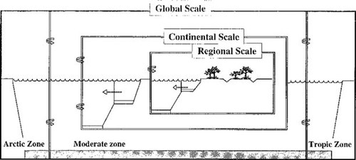
SimpleBox illustration of nested geographic scales. The innermost box is the regional scale containing 10 compartments. It is surrounded by the continental box containing 10 compartments as well. The arrows indicate air and water exchanges between scales. The two innermost boxes are contained within the global scale [3].
MODEL SELECTION AND TRANSFORMATION

The model is described as nested because it consists of three geographic scales, as illustrated in Figure 1. Here it is shown in its generic form with the regional scale within the continental scale, which is in turn nested within the global scale. The regional and continental scales consist of 10 well-mixed homogenous compartments including air, freshwater, seawater, freshwater sediment, marine sediment, three soil compartments, and two vegetation compartments. The global scale consist of only four environmental compartments: air, water, soil, and sediment. The species mass balance is applied to each compartment. At steady state, only the right side of the equation is used. For the three scales and the associated compartments, 24 equations yield as many chemical concentrations. Once the concentration are quantified all fate and transformation processes can be determined for the regional scale and beyond. With emission data, the nested attribute precludes having to arbitrarily estimate the numerous concentrations of the advective imports from the larger regions.
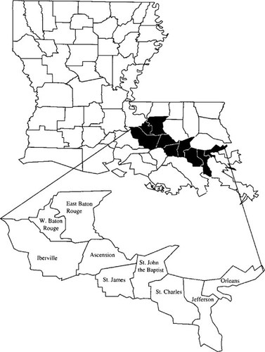
Modified geographical scales described in SimpleBox 2.0: industrial corridor, Louisiana, and continental United States. The industrial corridor is the innermost box; it is nested within the state of Louisiana and encompasses a nine-parish region along the Mississippi River between Baton Rouge and New Orleans (LA, USA). The state is in turn nested within the outermost box, which consists of the continental United States.
SimpleBox 2.0 was transformed to the Louisiana landscape and renamed LaCHEM for this specific application. The three generic geographic scales in SimpleBox 2.0 were modified as follows: the innermost regional scale became the chemical corridor, the continental scale became the state of Louisiana, and the global scale became the continental United States. Readers should consult the primary document [11] for the details of the landscape transformation. Figure 2 depicts the geographic scales defined in LaCHEM, and Table 1 gives the landscape characteristics. Because some are generic to all landscapes, several parameters were defaulted, or calculated using the SimpleBox algorithms. In LaCHEM, unlike the ideal scale juxtapositions illustrated in Figure 1, both the nine-parish region and the state are positioned on the edge of the United States global scale so that much of their advective output leaves the system. However, because of the relative area sizes of the inner scales the larger ones influence the smaller ones to a much higher degree than the reverse. Therefore, the inner-scale chemical loses are minor in affecting the magnitude of the respective background input concentrations. In addition, because the Mississippi River, USA, is leveed as it traverses the nine-parish region, it was not included in the freshwater flows. The levees divert all runoff away from the river and its flow does not flush through the corridor area so that including it would skew the regional freshwater residence time to unrealistic small values.
| Geographic scale | |||
|---|---|---|---|
| Characteristic (units) | Industrial corridor | State of Louisiana | Continental United States |
| Population (no. people) | 1,537,343 | 2,804,657 | NAa |
| Temperature (°C) | 20.1 | 15.5 | 12 |
| System area (land + water) (km2) | 5,362 | 123,233 | 9,629,091 |
| Area fraction water 1 (%) | 0.76 | 8.38 | 12.27 |
| Area fraction water 2 (%) | IE × 10−5 | 3.89 | NA |
| Area fraction soil 1 (natural) (%) | 48.88 | 22.03 | NA |
| Area fraction soil 2 (agricultural) (%) | 43.07 | 60.11 | 87.74 |
| Area fraction soil 3 (urban) (%) | 7.29 | 5.60 | NA |
| Height air (n) | 900 | 1,000 | 1,000 |
| Depth water 1 (m) | 0.5 | 0.5 | NA |
| Depth water 2 (m) | 25* | 200* | 1,000* |
| Depth sediment 1 (cm) | 3* | 3* | NA |
| Depth sediment 2 (cm) | 3* | 3* | 3* |
| Depth soil 1 (cm) | 18* | 17* | NA |
| Depth soil 2 (cm) | 20* | 20* | 5* |
| Depth soil 3 (cm) | 18* | 17* | NA |
| Wind speed (m/s) | 3.69 | 3* | 3* |
| Rain rate (mm/year) | 1,570 | 1,422 | 1,016 |
- a NA = not appropriate at this scale.
Chemical data
Two types of chemical data are needed as inputs for multimedia models: emission quantities into specific compartments and physicochemical properties. The rate at which a substance enters a particular environmental compartment is likely the most important input parameter. This information controls to a large degree the concentration through all media and it must be selected with great care. The following section, which is in reality a calibration exercise, describes its selection. Except for the degradation rate, most of the physicochemical properties are fixed and constant once the chemical is chosen, and sources are available [12-15]. The uncertainties in the decay half-life of the chemical within the primary compartment usually determine the range of predicted concentrations, thus contributing to its uncertainty. This aspect will be considered in a subsequent section.
Emission data
Three major databases contain emission information: The toxics release inventory (TRI), the toxics emissions database inventory (TEDI), and the national toxics inventory (NTI). The TRI includes data gathered from facilities required to report the amount of toxics released to the environment or transferred for disposal and contains industrial sources from the Standard Industrial Classification codes 29 through 41 for 300 pollutants [http://www.deq.state.la.us./oarp/airtox.htm]. The number of reportable pollutants in the TEDI is less, about 200, but it includes more industrial sources. Neither include mobile sources. The NTI includes a total of 796 unique point, area, and mobile sources; it contains 347 pollutants [http://epa.gov/pub/emisinventory/pei_96/ntist/la.txt] and is the most extensive database of the three. These represent primarily industrial manufacturing and use sources. For other sources, the search for data becomes chemical specific. The first four chemicals chosen were benzene, 1,1,1-trichloroethane (TCA), vinyl chloride, and atrazine. Benzene represents chemicals with mobile and industrial sources, whereas TCA and vinyl chloride are primarily of industrial origin. Atrazine is a herbicide often used on cotton and sugarcane crops grown in the industrial corridor [16]; its emission was estimated from agricultural databases [17; http://www.nass.usda.gov/census92/datafile/last/txt]. These four chemicals will be discussed in depth and are considered to be part of the model calibration process. Four additional chemicals from similar sources were chosen for the model validation process; these include toluene, trichloroethylene (TCE), styrene, and metribuzin.
The emissions inputs used, in units of 1,000 kg per year, for each chemical can be found in Table 2. Mobile sources are an important category for some chemicals. Reported mobile source data based on population [18] were added to the TEDI, which was used rather than the TRI because it contains more facilities. As will be discussed in the section on calibration, the search for comprehensive published emission data that would produce model concentrations in the range of measurements was a true calibration exercise.
Vinyl chloride originates from manufacturing facilities and all three databases contained similar quantities. The 1995 TRI was used because it contained data for all three geographic scales. The TCA is introduced from manufacturing facilities but also enters as end-use products (metal degreasing agents, paints, glues, household cleaners, aerosol sprays, and so on). The 1995 TRI data was used for TCA as well.
Atrazine is applied to the soil as a liquid mixture; application rates can vary depending on soil texture and climate. The application rate is 3 pints per acre (1.4 L/acre) per season [17]. The acres of sugarcane and cotton harvested in the industrial corridor, state of Louisiana, and United States [http://www.nass.usda.gov/census92/datafile/last/txt] are used to estimate the emissions.
| Scale | Benzene, TEDI + mobile | Vinyl chloride, TRI | TCE, TRI | Atrazine, estimated | Toluene, TEDI + mobile | Styrene, TRI | TCA, TRI | Metribuzin, estimated |
|---|---|---|---|---|---|---|---|---|
| Industrial corridor | 2,140 | 11 | 38 | 22 | 2,918 | 188 | 30 | 35 |
| State of Louisiana | 2,701 | 50 | 68 | 138 | 6,100 | 10 | 13 | 435 |
| Continental United States | 205,685 | 364 | 10,294 | 1,354 | 562,146 | 18,569 | 11,540 | 4,257 |
- a Abbreviated chemicals: TCE = trichloroethylene; TCA = 1,1,1-trichloroethane. Chemical emissions databases: TEDI = toxic emissions database inventory; TRI = toxic release index. One ton ∼2,200 pounds = 1,000 kg.
The emitted quantities for the four chemicals used in verification were done similarly. Toluene emissions include estimated mobile emissions plus those reported in the TEDI. The TCE and styrene emissions were obtained from the TRI and metribuzin was calculated based on application rates in the same manner as atrazine.
Degradation rates
Although SimpleBox contains algorithms for calculating degradation rates (Kdeg), literature values were used [12-15] and these are given in Table 3. When half-life, t1/2, information was available, pseudo–first-order degradation was assumed and calculated from the equation t1/2 = 0.693/Kdeg. If literature values were unavailable, the SimpleBox algorithm was used. Vapor pressure and solubility values are adjusted automatically by SimpleBox for temperatures other than 25°C. Average degradation rates were used in the model to obtain the outputs discussed in the following sections. However, in a later section, the entire range of reported values will be used to determine the sensitivity of this parameter on model-predicted concentrations.
Field measurements
Chemical monitoring data and other field-measured values were reported by the Louisiana Department of Environmental Quality (DEQ) for 1995 [19] and by the U.S. Department of Agriculture [20] for 1995 to 1997. The industrial corridor compartment is long, approximately 200 km, and narrow approximately 50 km, as shown in Figure 2. Distributed top to bottom, the parishes with sample location are: Baton Rouge with three air stations, West Baton Rouge with one water station, Iberville with two water stations, Ascension, and St. James with one air and one water station. The bottom four parishes, St. John the Baptist, St. Charles, Orleans, and Jefferson, contain no sample stations. Chemical sources are relatively evenly distributed along this corridor. Although the sampling sites are in the northern portion they are nonetheless generally representative of the compartment as a whole and suitable for model validation purposes. Because of the regulatory missions of these governmental agencies the data were assumed to be of high quality, reflecting state-of-the-art sampling and analytical chemistry protocols. No data from these published sources were rejected.
| Air | Water | Soil | ||||
|---|---|---|---|---|---|---|
| Chemical | Low | High | Low | High | Low | High |
| Benzene | 2.09 | 20.9 | 5.00 | 16.0 | 5.00 | 16.0 |
| Vinyl chloride | 0.40 | 4.04 | 28.0 | 180 | 28.0 | 180 |
| TCA | 225 | 2250 | 140 | 273 | 140 | 273 |
| Atrazine | Default | Default | Default | Default | 60.0 | 160 |
| Toluene | 0.42 | 4.33 | 4.00 | 22.0 | 4.00 | 22.0 |
| Styrene | 0.04 | 0.30 | 14.0 | 28.0 | 14.0 | 28.0 |
| TCE | 1.13 | 11.3 | 180 | 360 | 180 | 360 |
| Metribuzin | Default | Default | Default | Default | 30.0 | 120 |
RESULTS AND DISCUSSION
Studies performed with LaCHEM revealed that some parameters are highly constrained or relatively insensitive, whereas others were very sensitive for the predicted concentrations [11]. Parameter sensitivity analysis was performed by perturbating each over the expected range of variation and computing the concentration changes. These parameters included transport coefficients, physicochemical properties, degradation rates, wind and water speed, precipitation rates, and temperature. Changes occurred when steady-state temperature was varied to reflect seasonal changes. However, perturbations covering the range of published physicochemical properties, and variations of the estimated values of the transport coefficients, wind and water flow, and precipitation rates on a seasonal cycle did not cause significant (= 5%) concentration changes. The range of published values of Kdeg in the primary media were large and typically exceeded the range produced from the seasonal temperature variations of this parameter. In summary, in addition to the chemical source emission rate, EMIS in the equation, the sensitive parameters are Kdeg and, to a lesser degree, temperature. Therefore, these become the key adjustable parameter in the calibration process.
This section contains the results of the calibration phase demonstrating how the published emission and degradation data were used to bring predicted concentrations in line with the available monitoring data. The following procedure was used. Average literature values of the degradation rate were set in the model and the three emissions databases were used in turn to produce output concentrations. Graphs of the output concentrations were displayed on scatter plots of the monitoring data. As seen in Figure 3 for benzene, the graphs display concentration versus time. The time period for the data was the 1995 calendar year. Because the model is steady state, predicted concentrations appear as horizontal lines. The database that best represented the average concentration data was selected. The model was then run with maximum and minimum values of the literature-reported degradation rates. This produced a range of maximum and minimum model-predicted concentrations, which was superimposed on the monitoring data to visually assess the degree of overlap or the degree to which model predictions captured the data. This graphical approach provided a clear visual means of judging prediction versus data. Only minimal statistics involving average and standard deviation of measured concentrations were used.
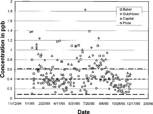
Predicted concentrations in air versus measured data showing sensitivity of degradation rates for benzene. Concentrations, in parts per billion (v/v), collected at the four sites within the industrial corridor for calendar year 1995 along with model-predicted concentrations are shown. The three horizontal lines superimposed on the data point are steady-state model predictions. Top to bottom the lines represent the maximum, average, and minimum benzene decay half-life in air; they are 20.9, 11.1, and 2.09 d, respectively.
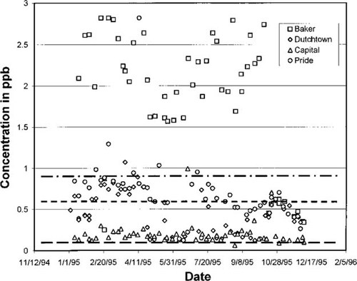
Predicted concentration in air versus measured data showing sensitivity to degradation rates for 1,1,1-trichloroethane (TCA). Concentration, in parts per billion (v/v), collected at four sites for 1995 along with predicted concentrations shown as horizontal lines. Top to bottom the lines represent steady-state model predictions based on maximum, average, and minimum TCA decay half-lives of 225, 1,238, and 2,250 d, respectively. The high concentrations at the Baker site suggest that it is near the source.
The calibration phase
Using the TRI database alone results in a projected benzene concentration in the corridor of 0.02 ppb. The average of the DEQ measurements is 0.528 ppb with a standard deviation of 0.354 ppb. When used alone, the TEDI and NTI databases also yielded concentrations significantly lower than the average of the measured data, 0.09 and 0.23, respectively. Including the mobile sources increased the projected concentrations by a factor of three for the NTI database and a factor of 16 for the TRI database, thus demonstrating their importance for benzene. The TEDI database plus mobile sources was accepted as the correct emission quantity because the model outputs represent a value close to the average of the DEQ data (0.398 vs 0.528 ppb).
The second element in the calibration phase was the selection of degradation rate constants. Sources for this parameter were reference works that contained reviewed and compiled information on numerous chemicals and that were derived predominately from laboratory studies. Ranges (i.e., maxima and minima) are shown in Table 3. The average is the arithmetic mean of these. Once the compartment that dominated chemical degradation loss was identified, its half-life was perturbed over the range. Benzene predicted concentrations ranged from 0.142 to 0.605, as seen in Figure 3. The monitoring data and standard deviation around the mean is 0.174 to 0.882 ppb. This constitutes a significant overlap.
The projected values for benzene generally are lower than the measured ones. This is to be expected because air samples at the four sites are near the ground where the sources are located. Likely travel times between chemical emission and capture by the sample apparatus is short; shorter than the air residence time in the assumed completely mixed air compartment of the corridor box. Alternatively, the release and capture occur in a portion of atmospheric layer of thickness less than the elevation of the air compartment, which is 900 m. In other words, the chemicals that are emitted into the box do not completely mix with the air mass within the compartment before sampling occurs. For these reasons, model predictions of chemical concentrations in the air compartment are expected to be lower than measured ones.
The predicted concentrations for TCA also overlap the measured data to a significant degree; these appear in Figure 4. The predicted concentration range was 0.163 to 0.967 ppb. The concentrations measured at the Baker monitoring site are significantly higher than the other three; the reason for this anomaly was never discovered. One plausible answer is that a larger number of industrial or commercial facilities producing or using TCA may be present very near the sample point. Vinyl chloride predicted concentrations are a factor of 10 lower than the measured ones; see Figure 5. The DEQ data include a significant amount of zero concentration readings resulting from limitations of the analytical chemistry protocols. The yearly average concentration including zeros is 0.02 ppb for the measured data and the predicted concentration range is 0.0022 to 0.0087 ppb. This factor of 10 difference may be the result of manufacturing emissions not captured by the TRI database, which was used for the emissions input. This difference may also reflect emissions from the lifecycle use of products containing vinyl chloride which are not accounted for in TRI database.
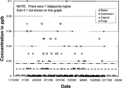
Predicted concentration in air versus measured data showing sensitivity to degradation rates for vinyl chloride. Concentrations, in parts per billion (v/v), collected at four sites for 1995 along with predicted concentrations shown as horizontal lines. Top to bottom the lines represent steady-state model predictions based on maximum, average, and minimum vinyl chloride decay half-lives in air of 4.04, 2.22, and 0.4 d, respectively. Measured data reflect one significant digit accuracy.
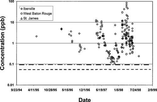
Predicted concentration in water versus measured data showing sensitivity to degradation rates for atrazine. Concentrations, in parts per billion (w/w), collected in three streams within the industrial corridor for calendar years 1995 to 1998 along with predicted concentrations are shown. Atrazine is applied periodically; however, the two horizontal lines are the steady-state model predictions where an equal continuous emissions rate is assumed. Top to bottom the lines represent soil decay half-lives; they are 160 and 110 d for the maximum and average values, respectively.
Projected concentrations for atrazine are shown in Figure 6 for the freshwater compartment. The three horizontal lines represent the concentrations computed from soil half-life of 60 to 160 d. Measured data were obtained from the U.S. Department of Agriculture for three of the nine parishes in the box: Iberville, West Baton Rouge, and St. James. All atrazine was applied to the soil. Although >99% remains there, atrazine nevertheless is water-soluble. Soil erosion is included as a model transport process so that when runoff occurs, a fraction enters surface water where it becomes easily sampled. Based on the degradation half-life, the predicted concentration ranged from 0.00751 to 0.091 ppb. The predicted high concentration is lower than the average measured data by more than a factor of 10, as seen in Figure 6. A log plot was used to encompass the variation in measured concentrations that occurs throughout the year. Of the chemicals used in this study, atrazine has the lowest solubility and highest octanol–water partition coefficient, so its high percentage association with soil is expected. It degrades fairly slowly in the soil, with half-lives of 60 to 160 d. This suggests that after it is applied some leaches into nearby water bodies. The concentration data shown in Figure 6 appear as streak lines, a term used to characterize high initial concentrations that decrease with time. This suggests a process of runoff resulting in an input pulse, followed by elimination or dilution in the receiving waters. South Louisiana water run-off was used; however, the data span three log scales and the model does not capture any of this data. The reasons are likely twofold. First, approximately one third of the water in the box receives atrazine; second, the applications, which occur nonuniformly for two to three months during the year are annualized. Both of these factors cause the model-projected steady-state concentrations to be lower than the measurements. Taken together expert-user corrections applied to the LaCHEM projections for atrazine suggest the output concentration should be higher by a factor of 10 or more. By assuming this, the model predictions capture the lower range of the measurements. The transient modeling option contained within SimpleBox may be more appropriate for atrazine in the smaller three-parish box. The use of the transient option would allow the accommodation of the application of atrazine in spring and fall input pulses, thus producing output concentrations in receiving waters that mimic the measured streak lines appearing in Figure 6. However, this aspect was not modeled.
The validation phase
Validation should provide useful information regarding the range of model applicability to various problem contexts such as different chemicals, geographic conditions, climatic conditions, sizes of the compartments used, and so on. In the case of the industrial corridor all these parameters are constrained except chemical type. Changing this one parameter is recognized to result in a less-than-robust validation exercise.
Four chemicals (toluene, styrene, TCE, and metributzin) were chosen to represent similar classes and sources as those used in the calibration exercise. Toluene, like benzene, is used in the petrochemical industries in the corridor and is also a component of vehicle emissions. Styrene is a common precursor used in the manufacture of plastics synthetic rubber, resins, and insulators. Upon exposure to light and air, styrene undergoes polymerization and oxidation with formation of peroxides [21]. The TCE is a common industrial solvent with emission origins similar to those of TCA. Metributzin is a triazine herbicide often used with sugarcane and other field crops; it matches atrazine in this regard. Physical and chemical properties and degradation half-life data were obtained from the literature; emissions data on each of these were taken from the same sources as used during the calibration process (see [11] for details). Predicted and measured concentrations of each were displayed as a function of time for 1995 so as to confirm the steady-state behavior and capture the degree of model versus data overlap. The toluene concentrations underpredicted the data by a factor of three. The data average was 0.72 ppb in air with a model value of 0.24 ppb using the average decay half-life of 2.38 d. When using the maximum to minimum degradation half-life, approximately 10% of the measured values were captured by the model. In the case of styrene, the measured average in air was 0.13 ppb and the model underpredicted by a factor of 45. No data were captured when the minimum degradation rate was used. Its degradation process in the environment is not well known and reactions in air are complex chain reactions so that a pseudo-first-order reaction rate equation is likely inadequate [21]. Model predictions for TCE (0.0055 ppb in air) using the average decay half-life were lower than the average measured value (0.04 ppb) by a factor of eight. Less than 10% of the data was captured by the model. Four measurements in water were located for metribuzin; they ranged from 0.24 to 0.58 ppb. Three were captured by the model predictions, with the average being 0.28 ppb.
Not surprisingly, the outcomes of the validation exercise were similar to those of the calibration exercise considering the nature of the chemicals employed. In almost all cases, the concentrations predicted were lower than measured values. However, only for styrene could the model results be judged incorrect. The most important parameter in achieving a high degree of correlation between predicted and measured concentrations is the correct emission rates of the specific chemical into the particular environmental media (i.e., air, water, soil, and so on). A high degree of correlation is defined as a significant overlap with the range of concentrations predicted by the model and the range of measured concentrations. This definition of measurements versus predictions is used in the following analysis.
The average predicted concentrations for benzene, metribuzin, and TCA adequately represent the measured average data, being low by a factor less than two. However, average vinyl chloride, toluene, and TCE concentrations were lower than the measured values by factors between 3 and 10. The likely reason is that all of the emissions sources are not accounted for in the databases used. The atrazine and styrene predictions by the model were substantially lower than the measured values. Factors for both were approximately 50. In the case of atrazine, its application mode was far removed from the steady-state ideal, whereas the complexity of the degradation process for styrene in air was not captured by the simple rate equation employed.
Conclusion
The goal of this study was to explore the possibility of using routine monitoring data for testing multimedia environmental models. The results show how this testing can be done and demonstrate the positive and negative outcomes along with the limitations of using monitoring data. For expert model users it provides a source of generally good-quality information for the calibration and testing of multimedia compartmental models. These users are keenly aware of the limitations of the model and the caveats that need to be included in interpreting its predictions. For example, it is now becoming clear from this and other studies that predicted concentrations given the correct emissions will nearly always be low. Even for substances with the correct degradation rates, transport and equilibrium parameters, and so on, and the correct media flows, mixing depths, and input into the model an underprediction of concentration in the primary media (i.e., that containing largest chemical mass) of a factor of 10 should be expected.
This is but a first tentative stab at the task of evaluating multimedia models and the validation approach taken is somewhat limited. Nevertheless, encouraged by these results additional studies employing monitoring data should be conducted in a variety of environmental settings with an expanded set of chemicals. The chemicals used in this study included six air-phase residers. Only two were in the water and soil, whereas none were in the sediment or plants. Hopefully in the future, monitoring data and corresponding emissions data can be located to further test these multimedia compartmental models. It will then be necessary to harmonize these monitoring and multimedia studies with the goal of extending their sphere of application and building confidence in their predictive abilities.
Acknowledgements
Support was provided by the Gordon A. and Mary Cain, Department of Chemical Engineering, Louisiana State University, Baton Rouge, Louisiana, USA.


