Demonstration of a toxicological risk ranking method to correlate measures of ambient toxicity and fish community diversity
Abstract
The goal of this study was to assess a new toxicological risk ranking model, field validate it with results from a battery of sediment and water column bioassays, and identify correlations of model output with fish community and population metrics. The model has five components: severity of effect, degree of response, bioassay variability, consistency, and number of measured endpoints. The model can reliably reduce an array of ambient toxicity data into a site-specific metric that is appropriate for comparisons with other metrics, such as Index of Biotic Integrity (IBI) or community diversity indices. The model is tolerant of variable amounts of data between stations. It does not generate probability limits without repeated sampling. The model can identify trends between sampling stations and document where chemical contamination is contributing to community impacts as well as where toxicological impacts are not likely to be contributing to observed population level impairment. The model was evaluated with field/laboratory data. Test sites were located in tributaries of Chesapeake Bay watersheds that are impacted by industrial, urban, and agricultural land use patterns. The toxicological risk scores correlate with fish community health metrics. The strongest correlations were between sediment toxicity risk and bottom trawl fish community diversity index.
INTRODUCTION
The goal of this study was to assess a new toxicological risk ranking model, field validate it with results from a battery of sediment and water column bioassays, and identify correlations of model output with fish community metrics. This project represents the initial attempt by the Maryland Department of Natural Resources (DNR) to integrate an environmental ambient toxicity testing scheme with a biological community assessment approach. The toxicological approach was designed to be applicable to assessing tributary-wide contaminant impacts or site-specific assessments. This paper describes the toxicological risk ranking model developed specifically for evaluating the results of tributary-specific ambient toxicity testing. The fish community metrics employed were measures of diversity and Index of Biotic Integrity (IBI). The ambient toxicity tests were laboratory-based bioassays using standard and/or local species. The details of the bioassays and metrics are not dealt with here.
The current approach was undertaken to further our understanding of how toxic contaminants may be affecting habitat quality and resource populations in Chesapeake Bay. The ultimate question to address is: To what extent do toxicants affect living resource populations in Chesapeake Bay? This is a very difficult question to answer in any coastal system with the current state of knowledge. A major difficulty exists in separating natural population fluctuations from anthropogenic factors.
Many species that depend on the Chesapeake Bay habitat for reproduction are in a more advanced state of decline than those that spawn outside the Bay [1]. Clearly, this effect is due to overharvest and/or loss of habitat or access to spawning grounds in some cases. It is also clear that some areas are severely contaminated and others demonstrate localized ambient toxicity [2-4]. It is unknown if localized toxic contaminant effects can influence populations in the Bay as a whole, or if low-level but widespread contamination is a greater problem, or if a combination of the two is important.
As a starting point in addressing the impact of toxic contamination on populations, the risk ranking method was developed to quantify ambient toxicological effects for statistical contrasts with biological community response parameters. The risk ranking model output can be contrasted with any type of community health metric, not just fish community metrics. Confirmation of deleterious effects at the community level is an inherent confirmation that population level effects are occurring. Positive correlation of toxicological impact and depressed community metrics implies cause and effect, but does not substantiate it without a demonstrable mechanism.
This approach is built upon efforts to demonstrate the presence of toxic contaminants in specific sites and regions. An ambient toxicity pilot program, sponsored by the DNR and the United States Environmental Protection Agency (EPA) Chesapeake Bay Program, field validated a suite of sensitive lethal and sublethal bioassays for resident aquatic organisms [3, 4]. The approach assumes that biologically significant environmental contamination is not necessarily predictable based solely on chemical analysis. Contaminants may be present but not bioavailable, or biological impacts may be occurring due to unmeasured constituents and synergistic interactions. It has been demonstrated that the bioassays have the ability to detect the presence of toxic effects in contaminated areas, in areas of unknown quality, and in areas previously thought to be pristine.
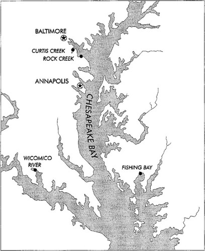
Map of Chesapeake Bay showing the location of rivers selected for joint ambient toxicity/Index of Biotic Integrity (IBI) sampling in 1993.
MATERIALS AND METHODS
Site selection
Previous studies [5-8] developed an estuarine fish IBI. Based on these studies, four tidal tributaries were selected for paired ambient toxicity/fish IBI sampling (Fig. 1).
Curtis Creek is a tributary of the Patapsco River in Anne Arundel County near Baltimore, Maryland, USA. The watershed is dominated by urban and commercial development. It was selected as an example of a polluted area to allow field assessment of existing test methods for ambient toxicity testing and the toxicological risk ranking model. Adverse biological effects expected at this site provided a positive control.
Rock Creek is also a tributary of the Patapsco River. The watershed is dominated by urban development with forested areas near the headwaters. It is also densely populated but with no heavily industrialized areas, as in Curtis Creek.
Fishing Bay is located in a lightly developed area of the eastern shore. The watershed is more than 70% forest and wetlands. It is the least urbanized of the study areas. Fishing Bay was thought to be a relatively unspoiled environment; however, the number of species caught in Fishing Bay had a similar pattern to that of stressed tributaries [6].
The Wicomico River is a tributary to the Potomac River, located between Charles and St. Mary's counties. This watershed contains the largest proportion of agricultural land of the four tributaries (approximately 30%, crop and pasture). There is little urban development, and forest and wetland occupy more than 50% of the watershed. The Wicomico served as the saltwater reference tributary in Carmichael et al. [5, 6]. The Wicomico River was selected to represent a relatively unimpacted reference area based upon consistently high IBI scores.
Field sampling and bioassays
Fish IBI sampling methods were designed to assess the fish community at its peak diversity in late summer. Tributaries were sampled three times each summer at two to five evenly spaced stations established along the axis of each tributary from its mouth to near the head of tide with beach seines and bottom trawls, deployed near mid-channel. The sampling stations were located beyond the direct influence of point sources. Ambient toxicity testing was initiated before the fish community IBI sampling was begun. This was done to assess the potential impact of toxic contamination as the fish communities matured to peak development and to assess any short-term spikes in toxic effects that may be detectable during the late spring and summer. Monthly, depth-integrated water samples were collected from the central trawl station in each tributary. Water column ambient toxicity bioassays were conducted monthly from May through September 1993 using a 7-d sheepshead minnow (Cyprinodon variegatus) survival and growth test and a 7-day grass shrimp (Palaemonetes pugio) survival and growth test at the DNR's Aquatic Toxicology Laboratory (Glen Burnie, MD, USA). Copepod (Eurytemora affinis) life-cycle survival and reproduction tests were conducted at the University of Maryland, Chesapeake Biological Laboratory (CBL) in July.
Sediment samples were collected with a petite ponar grab sampler at each fish community assessment trawl sampling station. The top 2 cm were retained for testing. Five sites were sampled in the Wicomico River and Fishing Bay. Due to their small size, Curtis Creek and Rock Creek only had two sampling locations. In these systems, two discrete samples were taken at the upstream sites, and three at the downstream sites. Sample sites were separated by ∼ 100 m on a linear or triangular sampling pattern. The sampling plan does not normally provide for true field replication for statistical purposes, but does allow a contrast of upstream versus downstream in the two smaller creeks. The rationale was the assumption of low temporal variation in sediment relative to the water column, and for the purpose of examining sediment contamination effects on a system-wide basis, which is consistent with the IBI community approach. This approach also allowed for an assessment of sediment contamination impacts on bottom communities and could be contrasted with benthic community metrics as well as bottom trawl survey data. Samples were segregated throughout the collection and toxicological tests.
Sediment toxicity bioassays were conducted using the following tests: 10-d sheepshead minnow (C. variegatus) embryo-larval survival and teratogenicity test; 20-d amphipod (Lepidactylus dytiscus) survival, growth, and reburial test; 20-d amphipod (Leptocheirus plumulosus) survival, growth, and reburial test; and 20-d polychaete worm (Streblospio benedicti) survival and growth test. Sediment bioassays were conducted by Old Dominion University, Applied Marine Research Laboratory (AMRL).
Culture and water column bioassay procedures for grass shrimp and sheepshead minnow were adapted from standard methods from the American Public Health Association (APHA) and the EPA [9, 10]. Copepod bioassays used methods modified from Hartwell et al. [11]. Culture and sediment bioassay procedures for the amphipods, polychaetes, and fish eggs were adapted from methods contained in Lambertson and Swartz [12] and DeWitt et al. [13]. Statistical evaluations for L. dytiscus were adjusted for particle size effects [3].
Heavy metals and acid and base/neutral extractable semivolatile organic compounds were analyzed on August water samples and bulk composite sediment samples using standard EPA methods. Total petroleum hydrocarbons in sediment were also measured by EPA method 3550 [14]. Inorganic contaminants were evaluated concurrently with sediment toxicity tests on a composite of the five discrete samples from each river system. Sediments were analyzed for acid-volatile sulfides and simultaneously extractable metals (AVS/SEM) using the method of DiToro et al. [15] and total organic carbon (TOC). Pore-water samples were extracted by squeezing with a nitrogen press and analyzed for ammonia, nitrite, and sulfides. Detailed methods and results of the bioassays can be found in Hartwell et al. [16]. The data were used here to test the risk ranking model.
Ranking model
At the inception of the ambient toxicity program, a ranking scheme was proposed to evaluate the toxicological results on a site-by-site basis [17]. The goal of the ranking system was to quantify the toxicological risk to populations due to the presence of toxic contamination, not merely to catalog presence or absence of toxic effects. The word risk is used here in the sense of jeopardy. If the toxicological risk score is high, due to high impact or high uncertainty, that implies resource populations in the test area are in more danger than areas with low impact or uncertainty. The model is not designed to replace a classical risk assessment, but may be a useful component of, or a companion to, the hazard or exposure assessment components. It specifically addresses ecological impact, without the necessity for demonstrating detailed, chemical-specific cause-and-effect relationships, which is one of the greatest difficulties in ecological risk assessment.
This scheme has five components: severity of effect, degree of response, test variability, site consistency, and number of measured endpoints. Each site was ranked by the following scheme. For each bioassay, endpoint severity was multiplied by the percent response of the test organisms for each bioassay endpoint, and the coefficient of variation for that test endpoint. This product from all bioassays was summed for each test site. The sum was adjusted by a site consistency factor and divided by the square root of the number of test endpoints (N) for each site, to compensate for bias between different sites where different amounts of data may be present.

Severity refers to the degree of effect that the bioassay endpoints measure. Mortality is considered the most severe response, followed by impaired reproduction and impaired growth. Other endpoints could be included in the list. The magnitude of the values and the relationship between them (e.g., linear, quadratic) needs further evaluation with empirical data. However, to evaluate the behavior of the model, the values of the endpoints were arbitrarily set as integers of mortality = 3, reduced fecundity = 2, and reduced growth = 1, and used consistently throughout.

Variability was expressed as the coefficient of variation (CV) of response for each set of laboratory replicates for each sample site. This parameter reflects the bioassay-specific variability for each endpoint and sample period. Thus, high variability may result in increased risk scores to a similar extent as positive toxic responses. Data were pooled by river or sample date in some cases for this purpose. It is recognized that this measure of variability may incorporate both experimental and site-specific variation between discrete samples. Experiments are currently underway to address this issue.
Severity, response, and variability are characteristics of the individual bioassays conducted at each site whereas consistency and the number of endpoints measured are site-specific attributes. Consistency refers to the agreement between the various bioassay endpoints measured at a site. If the results from all tests and/or species agree, consistency is high, and confidence in predicting toxic impacts (or lack of effect) is high. If half of the results are positive and half are negative, consistency and certainty of toxic impacts (or lack of impact) are lower.
Consistency was calculated as the cube of the difference between one-half the number of endpoints and the number of statistically nonsignificant responses at each site. Statistical significance in this instance refers to typical pairwise comparison tests of control versus experimental data, not a statistical test of the calculated response values from the equations above.

When bioassay endpoint values tend to be nonsignificant (N/2 ⩽X), the function is negative. When half of the endpoints are significant and half are nonsignificant (N/2 = X), the function is zero. When more than half of the endpoint values are statistically different from control values the function is positive. The absolute value is dependent on the amount of data available. Large data sets (high N) will have higher extremes. This polynomial function is an additive factor in the equation. The function reduces the risk score of a station when most of the test results were not significantly different from controls but increases the risk score when more than half the tests are significant.
| River | Bottom index | Resident index | IBI | Water risk | Sediment risk | Combined risk |
|---|---|---|---|---|---|---|
| Curtis Creek | 0a | 0.865 | 29.0 | 21.04 | 137.20 | 158.45 |
| Rock Creek | 1.428 | 1.761 | 35.0 | 17.90 | 76.48 | 47.02 |
| Fishing Bay | 1.760 | 1.086 | 28.5 | 10.46 | 58.24 | 24.73 |
| Wicomico River | 1.609 | 1.243 | 33.8 | 15.20 | 56.09 | 42.28 |
- a No fish were caught.
The number of endpoints measured at each site refers to the number of bioassays (species) and measured parameters (survival, growth, etc.) that are monitored. For statistical and experimental reasons, the number of tests run at each site ideally should be the same. However, given the uncertainties of experimental work, this is not always possible. For example, if mortality is very high, it may not be possible to measure growth.
A simple toxicity score can also be calculated for each discrete sample site. This is the sum of the products of endpoint severity and percent response divided by √N. Toxicity score = {Σ [(severity)(% response)]}\√N.
This score is a useful technique for comparing individual sites and for examining spatial trends in sediment or temporal trends in water samples. These calculations are also instructive in examining the response of the full risk ranking model and its response to inclusion of the interrelated factors of consistency and variation.
Data analysis
There are three possible risk ranking scores that may be calculated from the resultant data; water only, sediment only, or water and sediment combined. Because water column bioassays are replicated in the laboratory, a risk score can be calculated for each sampling month and the response scores can be averaged by river over months. This approach allows for an assessment of water column contamination effects on pelagic communities or possibly correlation to the abundance of specific species. Sediment samples were collected and tested as discrete samples without laboratory replication due to budgetary constraints. Therefore, calculation of a risk score can only be done by pooling the data together by tributary to calculate the CV and consistency factors.
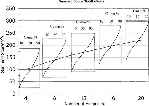
Plot of mean score generated by 1,000 random simulations of Σ [(severity)(response)(coefficient of variation)]. Insets show cumulative frequency distribution of potential summed scores at selected values of N (number of endpoints).
Sediment and water data may be combined together by river system to calculate a toxicity risk factor for the whole system. This calculation allows an assessment of toxic contamination on the entire river system with equal weight given to sediment and water column (assuming equal data availability). It also has the advantage of combining the data into larger subsets, which tends to dampen out individual spikes in the data set, without eliminating them. To pool the water data by river, the calculated response results were averaged over months. The CV of the mean responses was used in the risk calculation, rather than the mean CV value. Consistency was calculated as before.
The risk scores were contrasted to fish community IBI values. In addition, the Margalef [18] diversity index for bottom trawl community data and resident species (estuarine spawners) was calculated from the fish data.
Pearson correlation coefficients were calculated for every combination of toxicological risk score (water, sediment, and combined) and IBI, bottom trawl species diversity, and resident species diversity (Table 1). The resident species data included both bottom trawl and beach seine data but the value is dominated by species captured in the beach seines. The IBI score effectively incorporates all resident and migratory species in both the trawl and beach seine data. Calculation of an IBI score with only the trawl data would not be effective because it would incorporate an incomplete set of species, relative to the number of metrics in the IBI derivation. The IBI is designed to reflect the diversity and trophic structure of the entire fish community. This also means that the IBI score should respond to a variety of factors in the habitat, including, but by no means limited to, toxic impacts.
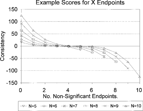
Plot of the range of possible consistency parameter values versus the number of nonsignificant endpoints for N = 5–10 (where N is number of endpoints).
RESULTS
The behavior of the model relative to the components of the summed products of response, severity, and variability is illustrated in Figure 2. Computer simulations were run to determine the potential range and distribution of values resulting from random combinations of response (0-100%), coefficient of variation (0-1.0), and severity (1, 2, or 3). Simulations were run at a number of endpoints (N) of 4, 8, 12, 16, and 20 to assess how the model responds to different amounts of data. One thousand simulations were run at each level and the cumulative frequencies of resulting products were tabulated. As the number of endpoints increases, the mean of the summed components increases linearly. The lower bound of values at N = 20 falls well within the range of even the N = 4 results. Thus, a small difference of one or two endpoints between stations is not likely to greatly bias results toward stations with more data.
For a given response scenario, the behavior of the consistency factor is illustrated in Figure 3. In the example of the sediment bioassays, using four species and measuring two endpoints for each (N = 8), the maximum value of the parameter is ± 64. This maximum value, relative to the extremes of the potential toxicity scores, is relatively small. If all bioassays were statistically significant and response values were in the range of 80 to 90%, the sum of the toxicity scores could reach into the range of 1,000+. Conversely, where average responses are in the range of 10%, the sum of toxicity scores would be less than 200. A consistency adjustment of 64 would be potentially significant relative to summary scores from other sites in this case. In the case of combined water and sediment scores (with seven test species in this case, N = 14) the maximum consistency score is ± 343. At low-level responses, the consistency factor could be larger than the summed response scores. The consistency score increases rapidly as the number of endpoints increases. At an N of 20 the consistency value maximum is ± 1,000. Even at high response values (summed response values between 3,000 and 4,000), the consistency value may have a larger proportional impact on the final score than with smaller data sets.
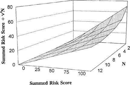
Plot of the effect of dividing the summed score by √ N for N = 2–12 (where N is number of endpoints).
The impact of division by √ N is illustrated in Figure 4. The influence is straightforward. All things being equal, sites with more measured endpoints will tend to have higher scores. Division by √ N partially corrects for this bias. If two stations had the same summed score, but a differing number of endpoints, the reason must be due to higher response and/or variability levels in the bioassay data from the site with less data. It is logical, therefore, for that site to have a risk score that reflects the risk of greater toxic impact. Division by √ N results in the final site risk score being higher for the site with fewer endpoints in this situation. Although this factor is primarily intended to counteract bias due to differing amounts of data at different stations, it also tends to moderate scores driven by extreme consistency factors. Extremely large (positive or negative) consistency factors by necessity will come from a high number of endpoints.
The behavior of the model was tested with toxicity data from the laboratory bioassays. Examples of bioassay results are included in Tables 2 to 4. These are included for illustrative purposes only, to show how the data were manipulated by the ranking scheme. The tables only reflect a portion of the database.
Briefly, the bioassay results demonstrated that statistically significant mortality or reduced growth did not occur in the water column bioassays. Growth rates were variable between sampling months at a given station, but with no apparent pattern. In the July copepod assays, survival to adult stages was significantly reduced in Curtis Creek relative to controls and the other stations. The Fishing Bay assay had very low survival and reproduction in both ambient and reference water, which was attributed to relatively high test salinities (11 ppt), to which the stock cultures were not adequately acclimated. Reproduction was lowest in Curtis Creek and Rock Creek.
| Site | Species | Endpoint | Severity | % Response | CV | Significant | Subscore | No. endpoints | No nonsignificant | Consistency | Risk score |
|---|---|---|---|---|---|---|---|---|---|---|---|
| CC | Eurytemora affinis | Mortality | 3 | 86 | 0.22 | Yes | 55.73 | 6 | 5 | -8 | 57.18 |
| CC | E. affinis | Reduced reproduction | 2 | 79.2 | 0.53 | 83.16 | |||||
| CC | Cyprinodon variegatus | Mortality | 3 | 0 | 0 | 0 | |||||
| CC | C. variegatus | Reduced growth | 1 | 0 | 0.24 | 0 | |||||
| CC | Palaemonetes pugio | Mortality | 3 | 0 | 0.87 | 0 | |||||
| CC | P. pugio | Reduced growth | 1 | 23.97 | 0.38 | 9.18 | |||||
| FB | E. affinis | Mortality | 3 | ND | 4 | 4 | −8 | 6.65 | |||
| FB | E. affinis | Reduced reproduction | 2 | ND | |||||||
| FB | C. variegatus | Mortality | 3 | 3.3 | 1.41 | 13.99 | |||||
| FB | C. variegatus | Reduced growth | 1 | 5.8 | 1.26 | 7.29 | |||||
| FB | P. pugio | Mortality | 3 | 0 | 1.73 | 0 | |||||
| FB | P. pugio | Reduced growth | 1 | 0 | 1.67 | 0 |
Chemical analyses of water samples did not reveal detectable semivolatile organic compounds, chlorinated pesticides, or polychlorinated biphenyls (PCBs) at any station. Of the metals, only silver was detected at elevated levels in Curtis Creek, Rock Creek, and Wicomico River samples (26, 21, and 28 μg/L [total], respectively).
Sediment bioassay results from Curtis Creek, Rock Creek, and the Wicomico River demonstrated elevated mortality of L. dytiscus. Leptocheirus plumulosus and S. benedicti exhibited increased mortality in Curtis Creek sediments. The sheepshead minnow egg test produced significant egg and larval mortality at both Curtis Creek and Fishing Bay. No significant reduction in growth was observed for L. dytiscus for any of the test sites. Leptocheirus plumulosus displayed significant reduction in growth rate at Curtis Creek and Wicomico River sites, whereas S. benedicti demonstrated reduced growth at Rock Creek.
Chemical concentrations on composited sediment samples were below detection for all organic analytes in the Wicomico River and Fishing Bay samples. Curtis Creek and Rock Creek sediments were contaminated with high molecular weight polycyclic aromatic hydrocarbons (PAHs) (Table 5). Petroleum hydrocarbons were found at the highest levels in Curtis and Rock Creeks, with elevated levels in Wicomico River sediments also, relative to Fishing Bay. All pore water SEM heavy metal levels in Curtis Creek and Rock Creek were high relative to Fishing Bay and Wicomico River (Table 6). Heavy metal concentrations in pore waters were an order of magnitude lower in Fishing Bay sediments and below detection in Wicomico River sediments, except for low levels of zinc.
| Site | Species | Endpoint | Severity | Response | Subscore | N | Score |
|---|---|---|---|---|---|---|---|
| CC | Lepidactylus dytiscus | Mortality | 3 | 58.21 | 174.63 | 8 | 157.02 |
| CC | L. dytiscus | Reduced growth | 1 | 0 | 0 | ||
| CC | Leptocheirus plumulosus | Mortality | 3 | 6 | 18 | ||
| CC | L. plumulosus | Reduced growth | 1 | 43.6 | 43.6 | ||
| CC | Streblospio benedicti | Mortality | 3 | 51 | 153 | ||
| CC | S. benedicti | Reduced growth | 1 | 30.88 | 30.88 | ||
| CC | Cyprinodon variegatus | Mortality | 3 | 4 | 12 | ||
| CC | C. variegatus | Reduced hatch | 3 | 4 | 12 | ||
| FB | L. dytiscus | Mortality | 3 | 0 | 0 | 7 | 64.31 |
| FB | L. dytiscus | Reduced growth | 1 | ND | |||
| FB | L. plumulosus | Mortality | 3 | 0 | 0 | ||
| FB | L. plumulosus | Reduced growth | 1 | 0 | 0 | ||
| FB | S. benedicti | Mortality | 3 | 0 | 0 | ||
| FB | S. benedicti | Reduced growth | 1 | 38.16 | 38.16 | ||
| FB | C. variegatus | Mortality | 3 | 44 | 132 | ||
| FB | C. variegatus | Reduced hatch | 3 | 0 | 0 |
The water column risk scores for each sampling period are shown in Figure 5. Values varied from slightly negative to above 50 depending on month. The spike in Curtis Creek in July is primarily due to E. affinis mortality and reproduction effects. The spike in June in the Wicomico River is entirely due to fish growth data. Pooled risk values are shown in Figure 6. With a larger database, the overall Wicomico River risk score becomes a much lower value due to a lower consistency value.
The sediment risk scores are shown in Figure 7. Again, the Curtis Creek score is higher than any other station. The individual toxicity scores for discrete sediment samples are shown in Figure 8. The values vary widely from site to site. Recalling that the Curtis Creek and Rock River stations consisted of only upstream and downstream stations, it is obvious that the downstream Curtis Creek location accounts for the vast majority of the response score. A t test of the toxicity scores from the upstream versus downstream Curtis Creek sites was significant in a one-tailed test (t = 2.47, 3 d.f., p = 0.05).
| Site | Medium | Species | Endpoint | Severity | % Response | CV | Significant | Subscore | No. endpoints | No nonsignificant | Consistency | Risk score |
|---|---|---|---|---|---|---|---|---|---|---|---|---|
| CC | Sediment | Lepidactylus dytiscus | Mortality | 3 | 52.08 | 0.26 | Yes | 40.62 | 14 | 9 | -8 | 149.65 |
| CC | Sediment | L. dytiscus | Reduced growth | 1 | 0 | 0 | 0 | |||||
| CC | Sediment | Leptocheirus plumulosus | Mortality | 3 | 22 | 1.02 | Yes | 67.32 | ||||
| CC | Sediment | L. plumulosus | Reduced growth | 1 | 44.67 | 0.63 | Yes | 28.14 | ||||
| CC | Sediment | Cyprinodon variegatus | Mortality | 3 | 44 | 0.94 | Yes | 124.08 | ||||
| CC | Sediment | C. variegatus | Reduced hatch | 3 | 7.2 | 0.8 | 17.28 | |||||
| CC | Sediment | Streblospio benedicti | Mortality | 3 | 19.6 | 1.41 | 82.91 | |||||
| CC | Sediment | S. benedicti | Reduced growth | 1 | 26.13 | 1.01 | 26.39 | |||||
| CC | Water | Palaemonetes pugio | Mortality | 3 | 4.58 | 1.65 | 22.75 | |||||
| CC | Water | P. pugio | Reduced growth | 1 | 13.84 | 0.57 | 7.93 | |||||
| CC | Water | C. variegatus | Mortality | 3 | 3.17 | 1.22 | 11.63 | |||||
| CC | Water | C. variegatus | Reduced growth | 1 | 0 | 2.68 | 0 | |||||
| CC | Water | Eurytemora affinis | Mortality | 3 | 86 | 0.22 | Yes | 55.73 | ||||
| CC | Water | E. affinis | Reduced reproduction | 2 | 79.2 | 0.53 | 83.16 | |||||
| FB | Sediment | L. dytiscus | Mortality | 3 | 8.87 | 1.82 | 48.43 | 12 | 11 | −125 | 23.03 | |
| FB | Sediment | L. dytiscus | Reduced growth | 1 | 3.16 | 1.41 | 4.46 | |||||
| FB | Sediment | L. plumulosus | Mortality | 3 | 9.8 | 0.54 | 15.88 | |||||
| FB | Sediment | L. plumulosus | Reduced growth | 1 | 1.5 | 1.24 | 1.86 | |||||
| FB | Sediment | C. variegatus | Mortality | 3 | 31.2 | 0.77 | Yes | 72.07 | ||||
| FB | Sediment | C. variegatus | Reduced hatch | 3 | 3.6 | 1.51 | 16.31 | |||||
| FB | Sediment | S. benedicti | Mortality | 3 | 2.6 | 1.62 | 12.64 | |||||
| FB | Sediment | S. benedicti | Reduced growth | 1 | 19.86 | 1.11 | 22.04 | |||||
| FB | Water | P. pugio | Mortality | 3 | 0.21 | 9.95 | 6.21 | |||||
| FB | Water | P. pugio | Reduced growth | 1 | 0 | 3.69 | 0 | |||||
| FB | Water | C. variegatus | Mortality | 3 | 2.99 | 0.54 | 4.89 | |||||
| FB | Water | C. variegatus | Reduced growth | 1 | 0 | 1.47 | 0 | |||||
| FB | Water | E. affinis | Mortality | 3 | ND | |||||||
| FB | Water | E. affinis | Reduced reproduction | 2 | ND |
The risk scores for combined water and sediment data are shown in Figure 9. The basic patterns seen in the water and sediment scores are reflected in the combined scores. The score from the Curtis Creek site is more than twice as high as that of any other station. Fishing Bay had the lowest risk score. Because the risk calculations do not produce quantified measures of variability, there is no way to test one site against another statistically in the Wicomico River and Fishing Bay data.
| Site | |||||
|---|---|---|---|---|---|
| Chemical | Curtis Creek | Rock Creek | Fishing Bay | Wicomico River | NOAA ER-L |
| Fluoranthene | 540 | 480 | BDLa | BDL | 600 |
| Pyrene | 510 | 420 | BDL | BDL | 350 |
| Chrysene | 300 | 290 | BDL | BDL | 400 |
| Benzo[a]anthracene | 220 | BDL | BDL | BDL | 230 |
| Benzo[b]fluoranthene | 320 | 290 | BDL | BDL | NAb |
| Benzo[k]fluoranthene | 300 | 380 | BDL | BDL | NA |
| Benzo[a]pyrene | 250 | BDL | BDL | BDL | 400 |
| Petroleum hydrocarbons (mg/kg) | 509 | 680 | 180 | 428 | NA |
- a BDL = below detection limit. b NA = data not available.
The correlation coefficients for the risk scores and the fish community metrics from 1993 are shown in Table 7. The bottom trawl diversity index was strongly correlated with the sediment toxicological risk score and the combined score, which was driven by the sediment score. The resident species diversity index and the overall IBI did not have strong correlations with the toxicological risk scores. The strong relationship between all the toxicological risk scores and bottom diversity index can be seen in Figures Fig. 10.-Fig. 12.. The resident species diversity index demonstrates a similar trend with bottom and combined risk scores, but they are not statistically significantly correlated.
| Site | Cadmium | Lead | Copper | Nickel | Zinc | Sum |
|---|---|---|---|---|---|---|
| Curtis Creek | 0.322 | 0.360 | 1.051 | 0.144 | 2.966 | 4.575 |
| Fishing Bay | 0.017 | 0.036 | 0.022 | 0.022 | 0.326 | 0.423 |
| Rock Creek | 0.057 | 0.383 | 0.870 | 0.292 | 4.403 | 6.006 |
| Wicomico River | 0.000 | 0.000 | 0.000 | 0.000 | 0.023 | 0.023 |
| Detection limits | 0.0003 | 0.0050 | 0.0006 | 0.0004 | 0.0005 |
- aMercury values for all sites were <0.001 μmol/g.
DISCUSSION
Overall, bioassay results indicate that the assays are sensitive enough to identify biologically significant contamination. The risk results demonstrate that water column toxicity is not as severe as localized sediment toxicity but that water column effects may be more widespread and variable over time. The risk ranking procedure results in comparable data sets between sites. For example, not all sites have the same number of tests. Growth could not be assessed in some Curtis Creek sediment tests due to high levels of mortality. This site ranked far above all other sites in spite of this, due to the relatively high consistency, high response rates, and that the observed effects were principally mortality, which has the highest severity factor. It is recognized that some of these values are arbitrary and need further refinement as more data become available.
Both severity and degree of response are straightforward parameters if only one type of bioassay is run at each test site. However, given a suite of tests run at each site, some system of factoring in the relative sensitivity of different species and different endpoints needs to be developed for these two parameters. Adjustment of degree of response by a simple division by the frequency of positive responses would bias the results toward those endpoints with low sensitivity. Also, a factor for sensitivity and severity must be carefully weighted, as they are likely to be confounded in response patterns. That is, endpoints that are severe (e.g., mortality) may be less sensitive than other endpoints. This may not always be the case, depending on the mode of action of the toxicants present in the environment and their synergistic interactions with the test species.
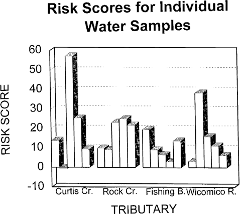
Risk scores for individual water column samples from four Chesapeake Bay tributaries evaluated for ambient toxicity in 1993. Individual bars from left to right represent results from May to September for each tributary.
The consistency factor can drive the score to be negative if there are a large number of endpoints and/or the response values are very low. The scoring method for toxicity ranking demonstrates site- and/or sample-specific differences between stations and sample times. Inclusion of factors for consistency and variability provides additional information for risk ranking of toxic impact, which is sensitive to the amount of data and the agreement between results from different bioassays.
No individual model parameter can be seen to drive the model output. Table 8 lists regression statistics for each parameter versus risk score. With one exception, correlation coefficients (r2) are low, which indicates weak relationships between final risk scores and individual parameter values. Thus, the model appears to incorporate all the parameters equally. Severity values should always be the same for all rivers, unless some endpoints are not measured in some systems. The slopes for response versus risk regressions were all significant. This is to be expected because higher response values should be reflected in higher risk scores. However, the correlation co-efficients were relatively low, indicating that the final risk scores reflect more than just the level of response. Observed bioassay coefficients of variability were inversely related to risk, but did not have a strong influence on the risk scores. Consistency is a result of the number of endpoints and the number of significant endpoints and consistency and N are therefore statistically confounded. When used as the test parameter, consistency appears to correlate strongly with risk score for combined data, but there were only four data points (from four bodies of water) and consistency would be expected to track with the final risk score because it is driven by the number of significant endpoints. Consistency does not correlate well with risk score in the water column data when calculated on a month-by-month basis (N = 20) and the r2 value for sediment (N = 4) is only 34%. The consistency factor was designed to act as a counterweight to response values for the purpose of damping out rare spikes, while not influencing scores from uniformly consistent response results. The consistency factor will tend to enhance the score of highly polluted sites and lower the scores of uncontaminated sites. The pooled risk scores for water and sediments from Curtis Creek are at least twice as high as the next nearest score. The consistency factor value for Curtis Creek was near zero. The values in the other sites were strongly negative. Stepwise regression [19] of severity, response, CV, and consistency with risk score identified response as the only significant factor in the water column data. Both response and consistency were identified as significant in the final stepwise model for the sediment data and only consistency was included in the model for the combined water and sediment data set.
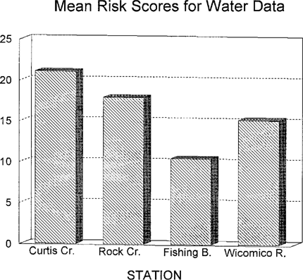
Mean risk scores for water column bioassay data from four Chesapeake Bay tributaries evaluated for ambient toxicity in 1993.
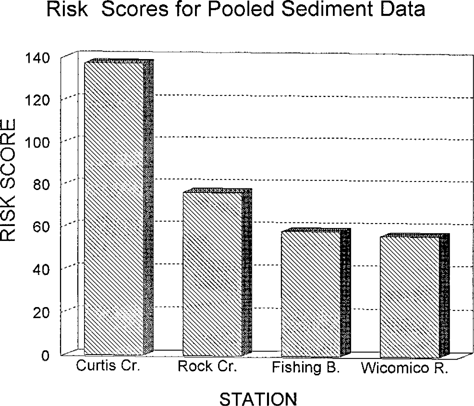
Risk scores for pooled sediment data from four Chesapeake Bay tributaries evaluated for ambient toxicity in 1993.
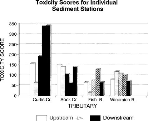
Toxicity scores for individual sediment samples from four Chesapeake Bay tributaries evaluated for ambient toxicity in 1993.
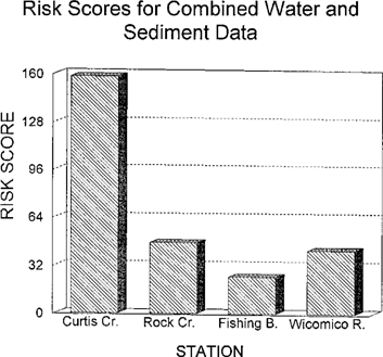
Risk scores for combined sediment and water data from four Chesapeake Bay tributaries evaluated for ambient toxicity in 1993.
Data are also included in Table 8 to contrast response scores versus variability. Biological response data have a tendency to have relatively higher variability at low and threshold effects levels. This does not appear to be a significant complication in this case.
The combined scores are not merely the sum of the sediment and water scores. Numerically, the combined Curtis Creek risk score is greater than the water or sediment scores. The combined Wicomico and Fishing Bay scores are in between their water and sediment values. The combined Rock Creek risk score remains at or above the individual water and sediment values, which may indicate some form of threshold value that integrates data volume and level of response in the model. Average response values were not greatly higher in Rock Creek than in Fishing Bay or the Wicomico River, but they were more consistent.
Some information is lost in the process of pooling the data to calculate a risk score on a river-by-river basis. For example, the copepod bioassays were not run as often as the other water column tests but they are given equal weight in terms of contribution to the final score because data are summed by river for each bioassay endpoint. This does have the advantage of smoothing out individual spikes in the data set. It is instructive, however, to look at the spikes by assessing risk scores (or toxicity scores in the case of sediment) on a sample-by-sample basis. This approach displays the occurrence of transient spikes in the Wicomico water column and the downstream gradient in Curtis Creek sediment toxicity.
| Risk score | IBI score | Bottom diversity index | Resident diversity index |
|---|---|---|---|
| Water risk | 0.1980 | -0.8290 | -0.0090 |
| (0.8023) | (0.1706) | (0.9908) | |
| Sediment risk | -0.3870 | -0.9910 | -0.4610 |
| (0.6126) | (0.0092) | (0.5387) | |
| Combined risk | -0.3790 | -0.9980 | -0.5490 |
| (0.6213) | (0.0018) | (0.4513) |
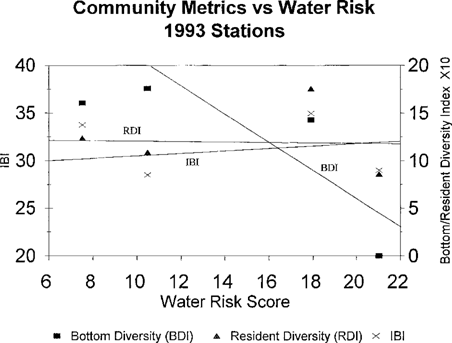
Mean risk scores for water samples from four tributaries of Chesapeake Bay sampled in 1993 versus fish community metrics. (Bottom diversity index, BDI; resident diversity index, RDI; Index of Biotic Integrity, IBI.)
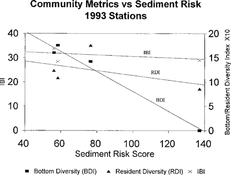
Pooled risk scores for sediment samples from four tributaries of Chesapeake Bay sampled in 1993 versus fish community metrics. (Bottom diversity index, BDI; resident diversity index, RDI; Index of Biotic Integrity, IBI.)
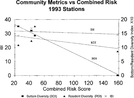
Combined risk scores for water and sediment samples from four tributaries of Chesapeake Bay sampled in 1993 versus fish community metrics. (Bottom diversity index, BDI; resident diversity index, RDI; Index of Biotic Integrity, IBI.)
It should be noted that the final risk ranking values should be interpreted with respect to specific results in laboratory data. The response scores for growth in the Wicomico River sediment bioassays can be attributed to grain size and/or TOC effects on both amphipod species. These effects tend to artificially increase the Wicomico River score slightly. In the case of Fishing Bay, there is no reproductive response score contribution from the E. affinis bioassays. This is due to the lack of acceptable control results. Therefore, the response score cannot be calculated, but reproductive failure is clearly indicated by the data for this system. Conversely, it is unknown if the fish egg mortality data are influenced by sediment ammonia levels. Pore-water levels were above lethal levels for sheepshead minnow larvae [20], but ammonia was not measured in the overlying water in the bioassays.
Finally, the sampling sites were not selected randomly. Curtis Creek is an area of known contamination problems. The toxicological ranking model clearly reflects this. Furthermore, the depauperate bottom fish community seen in the absence of a consistently anoxic condition indicates a chemical contaminant problem, especially in the sediment [6]. Water quality problems in Rock Creek may have as much to do with nutrient enrichment as with contaminants from urban runoff and marina operations [21]. The Wicomico River was considered to be relatively clean, but with potential agricultural runoff impacts. Fishing Bay has no history of contamination and the watershed is largely undeveloped.
| Parameter | Slope | r2 % |
|---|---|---|
| Water | ||
| Severity | 0.61 | 0.17 |
| Response | 0.33**a | 19.21 |
| CVb | -1.57 | 2.97 |
| Consistency | -0.16 | -0.64 |
| Response versus CV | -0.02 | 3.52 |
| Sediment | ||
| Severity | -1.18 | 0.12 |
| Response | 1.00** | 21.87 |
| CV | -22.27 | 11.87 |
| Consistency | 1.81 | 34.90 |
| Response versus CV | -0.01* | 18.03 |
| Sediment and water | ||
| Severity | -0.17 | 0.00 |
| Response | 1.04** | 16.93 |
| CV | -23.02 | 5.74 |
| Consistency | 1.00* | 92.86 |
| Response versus CV | -0.01 | 23.54 |
- a* Slope significantly different than 0 at P = 0.05; ** slope significantly different than 0 at p = 0.01.
- b CV = coefficient of variation.
The correlation between the toxicological scores and the IBI metrics are consistent with these interpretations. The risk scores are correlated with the trawl data, particularly the sediment risk scores, as opposed to the water column risk scores (Table 7). The resident species metrics were not well correlated with the risk scores. The definition of resident species as estuarine spawners is important in this regard. This metric is dominated by species taken in the beach seines in terms of number of species and individuals, particularly in Curtis Creek, where no fish were caught in the trawls in 1993. The “resident species” are thus not living in close contact with the sediment at the bottom of the channels where the sediment samples were taken. The toxicological data clearly demonstrate that sediment toxicity is a dominant problem in Curtis Creek, but that the water column scores were marginal there, as in all systems.
- 1.
Areas with high IBI scores and/or diversity indices will always have low toxicological risk scores, unless populations have adapted to contaminated conditions.
- 2.
Areas with high toxicological risk scores will always have low IBI scores and/or diversity indices, unless populations have adapted to contaminated conditions.
- 3.
Areas with low IBI scores and/or diversity indices may or may not have high toxicological risk scores, depending on the nature of the reason for poor fish communities.
As studies progress, more sites will be included in the analyses. The IBI database, which spans several years from specific locations, will be used to test these hypotheses as more ambient toxicity data become available.
Additional work needs to be done to examine how well the toxicological risk ranking results from different years can be integrated. In addition, an assessment is needed on the importance of sampling intensity, relative to the size of the river system, on toxicological risk score sensitivity.
Acknowledgements
Sediment bioassays and pore-water chemical analyses were conducted by Ray Alden, Pete Adolphson, and Joe Winfield. Copepod bioassays were conducted by David Wright, Gena Coelho, and John Magee. Invaluable field sampling assistance was provided by Margaret McGinty, Sandy Ives, Doug Randle, and Bill Rodney, under the direction of Stephen Jordan. Additional field assistance was provided by Randy Kerhin. Tyler Hartwell and Andy Clayton assisted with computer simulations for model sensitivity assessment.


