The probability-based granular field of vegetated soils
Funding information: Strategic Priority Research Program of the Chinese Academy of Sciences, Grant/Award Number: XDA23090202; National Natural Science Foundation of China, Grant/Award Numbers: 41790432, 41977257; Key Science and Technology Projects of Transportation Industry, Grant/Award Number: 2021-MS4-104; Sichuan Provincial Transportation Science and Technology Project, Grant/Award Number: 2021-A-08
Abstract
Soils in vegetation-covered areas are of high variability in space and time, and the variability is crucial for hydro-geophysical processes at small and large scales. Conventionally, the spatial heterogeneity at large scale is visualized as a regional division map of soil properties by extrapolating sample measurements. No formalized method is available for assigning parameters for soils at the resolution of a small grid cell. This study formulates a method of establishing parameter space for vegetated soil by a single index (μ) derived from the unified grain size distribution (GSD). The index μ varies in space as a random variable and defines soil as a granular field. The μ-division represents the concentration of fine grains in response to root–soil interactions. Coupling μ-division with moisture distribution suggests that the gradient of μ plays a potential role in rooted soil hydraulics. It is further found that μ satisfies the Weibull distribution, which makes it possible to establish the μ-field for a soil space at large scale using the random dataset of μ. A case study is conducted in two vegetated slopes based on high-resolution digital elevation models (DEM) derived from unmanned aerial vehicle survey to create the field and illustrate its implications in morphology and hydrology. It is expected that the μ-field may derive parameter fields of various soil properties as functions of the GSD parameters and thus equip DEM with a complete dataset of soil. The paradigm proposed in the study fills the gap of establishing high-resolution data space for soil at large scale for dynamics of surface processes.
1 INTRODUCTION
Soils in nature are inherently of high spatial variability at various scales. For vegetated soils, the variability is especially dramatic owing to the root–soil interactions. Complex vegetation patterns and diverse topography have produced and enhanced variability and heterogeneity (Burns et al., 2017; García-Palacios et al., 2012; Hendriks et al., 2015; Parker & Lear, 1996). Spatial variability plays special roles in influencing hydro-geophysical processes because of the crossing scales of problems. For examples, soil moisture is variable in time and space and impacts processes at scales ranging from point, hillslope, basin to global (Isham et al., 2005). At a small scale (from 1m2 to 1 km2), soil moisture is crucial for the infiltration process (Raats, 2001), plant dynamics (Porporato et al., 2001), and slope processes, while at large scale it impacts the hydrologic cycle from microscale (~1 km2) to large grid size (~104 km2) (Chahine, 1992).
Spatial variability of soil is usually represented by variance of soil properties (Duncan, 2000; Mori et al., 2020; Wu et al., 2020), with uncertainties due to limited availability of information and measurement errors (Baecher & Christian, 2005; Phoon & Kulhawy, 1999; Vanmarcke, 1977). Pedotransfer functions, for instance, are expressed in terms of textural classes (Vereecken, 1995; Wösten & van Genuchten, 1988) or matric potential (Contreras & Bonilla, 2018; Kern, 1995; Nemes & Rawls, 2006; Ungaro & Calzolari, 2001), which are obtained only by directly measuring individual samples in field or laboratory. When a large-scale area is concerned, establishing a data space requires a large number of samples and technique of data extrapolation (Brocca et al., 2010; Pachepsky et al., 2013). This is always time consuming, tedious, and expensive, in the absence of a universal operational algorithm.
Deriving soil properties from the routinely measured properties has long been an ambition (e.g., Gupta & Larson, 1979) and grain size distribution (GSD) plays a fundamental role (Arya & Paris, 1981; Ghosh, 1980; Rosas et al., 2014; Zhai et al., 2020). Various parameters, GSD functions, and probability distributions have been proposed for describing soils (Bird & Perrier, 2003; Folk & Ward, 1957; Hatheway, 1996; Hwang et al., 2002; Kondolf & Adhikari, 2000; Rubin & Topping, 2001; Zobeck et al., 1999) or estimating soil properties (Arya et al., 2008; Fredlund et al., 2000; van Genuchten, 1980). However, there is still the lack of an integrated index for soil characteristics.
Finding a way out of this difficulty is the aim of the present work. In this study, we propose a new method of establishing a random field using a single granular index derived from a unified GSD function. First, we introduce the scaling GSD function and the derived indicative exponent; then, we use the exponent to visualize the spatial variability of soil in root zones under the background of root–soil–water interactions; finally. we create the random granular field for vegetated slopes based on high-resolution digital elevation models (DEM) created from unmanned aerial vehicle (UAV) surveys. This attempt forms a new paradigm for granular analysis and provides a practical framework of parametrizing soil characteristics over an area at any scale.
2 FOUNDATION FOR THE GRANULAR FIELD OF SOIL
The GSD function is remarkable in having two advantages: it is universally applicable for a great variety of soils, irrespective of their sources, types, and textures; and it is dynamically preserved in that soils undergoing various processes retain the same distribution. Therefore, the GSD parameters not only feature the state of soil texture, but also represent soil changes in various processes. As (μ, Dc) varies in soil space, a soil behaves as a random field, which can be properly coined as “granular field”; then the hydraulic and geophysical processes of soil are associated with the evolution of the granular field. Furthermore, it is found that soil properties, both hydrologic and mechanic, can be expressed in terms of the GSD parameters—for example, X = f(μ, Dc) (Gou et al., 2015, 2021)—therefore, it is possible to derive other fields of dynamical parameters; for example, X may take cohesion (c), friction angle (φ), porosity (n), and hydraulic conductivity (Ks).
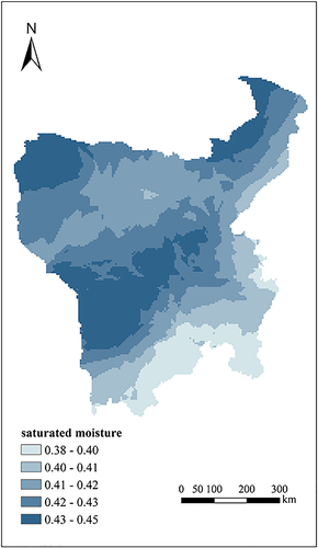
In comparison, the existing pedotransfer functions are usually expressed by a linear combination of textural parameters (Contreras & Bonilla, 2018), X = ∑aiψi, with ψi the percentage of texture class (e.g., clay, silt, and sand), organic content, and bulk density (Gupta & Larson, 1979; Homaee & Firouzi, 2008). The quantities ψi can be only obtained by directly measuring individual samples but cannot be integrated in a general operation framework. A huge dataset is required to build a parameter space on a large scale. In practice, one usually gets a regional division map of a soil property, as shown by Figure 1, which presents the saturated moisture distribution of the Hengduan Mountains (about 6.0 × 10⁵ km2) in southwest China, based on the national soil survey. Obviously, such division does not reflect the spatial heterogeneity at small scale, which is fundamental for local dynamical processes. To say the least, even when the dataset is sufficiently large, the parameter set {ψi} does not easily take the role of indicative indices for soil.
On the other hand, the GSD parameters are simple, formally derivable, and generally comparable; thus they are ready to take the indicative role. Because general soil character is almost entirely governed by fine content (Hatheway, 1996), we may use μ (representing fine fraction) as the single indicative exponent. The variation of μ features the soil variability, and the soil space is equipped with a structure of random μ-field. This forms the background to the study. In the following, we will use the GSD exponent to illustrate the spatial variability of soils and establish the parameter space for vegetated slopes, in a case study in southwest China.
3 CASE STUDY FOR ESTABLISHING THE μ-FIELD OF SOIL
3.1 Soil sampling and texture composing
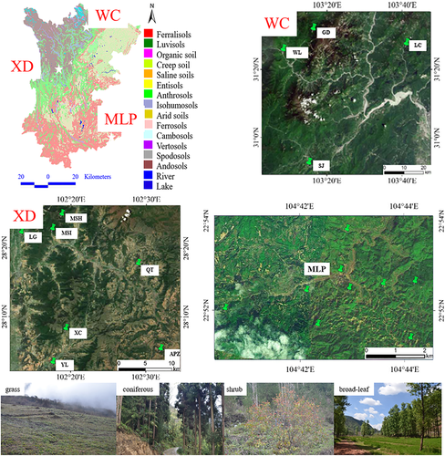
Twelve test spots in southwest China were selected for the study (Figure 2), where the complexity and adversity of topography, climate, vegetation, and soil, as well as the related surface processes (e.g., water–soil erosion, slope failures, landslides, and debris flows), are representative (Table 1). In order to obtain accurate DEM for building the data space, we have taken UAV (DJI Inspire 2 type drone) surveys in the areas, with flight of 260 m high, 3–5 m/s, and 10 Hz measurement, covering typical watersheds and hillslopes. Using the Agisoft PhotoScan, we can create DEM at a resolution of 0.7 × 0.7 m (dpi 960p and corresponding frame rate 30 fps).
| Soil type | Location (vegetation cover) | Vegetation combination | ||||
|---|---|---|---|---|---|---|
| Grass | Shrub | Broad-leaf | Coniferous | |||
| Yellow-brown soil | Wenchuan in Minjiang River Basin (WC) 40 × 4 × 5 = 800 samples | LC (Longchi) (69%) | Astilbe chinensis, Paspalum notatum | Euonymus szechuanensis | ||
|
MSI (Miansi) (28%) |
Notopterygium incisum, Phlomis umbrosa | Leucaena leucocephala | ||||
|
WL (Wolong) (45%) |
Crawfurdia sessiliflora, Dichanthium annulatum | |||||
|
GD (Gengda) (38%) |
Dodanaea angustifolia and Rhododendron rufum | |||||
|
SJ (Sanjiang) (21%) |
Cymbopogon distans, Heteropogon contortus | |||||
| Laterite, brown soil | Xide in Jinsha River (XD) 40 × 4 × 5 = 800 samples |
YL (Yiluo) (67%) |
Euonymus szechuanensis | |||
|
MSH (Mianshan) (78%) |
Pinus massoniana | |||||
|
LG (Lugu) (23%) |
Lonicera pileata, Rosa sericea | |||||
|
APZ (Apuzu) 43% |
Bothriochloa pertusa | Pinus massoniana | ||||
|
QT (Qietuo) (26%) |
Melinis minutiflora, Heteropogon contortus | Corylopsis willmottiae | ||||
| Brown soil |
Xichang by Reshuihe river (XC) 40 × 4 = 160 samples (76%) |
Artemisia simulans, Pedicularis nasturtiifolia | Betula utilis | |||
| Lateritic red soil |
Malipo in Yunnan (MLP) 40 × 15 = 600 samples (56%) |
Setaria glauca, Indigofera enneaphylla, Bothriochloa pertusa | ||||
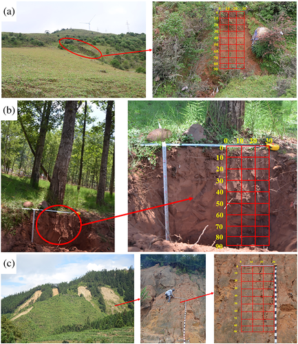
Soil samples (2360 in total) are collected in root zones and slopes (Figures 2 and 3, Table 1). The major root systems are shown in Figure 3. The grass Cynodon dactylon (L.) Pers. has a herringbone-like root system, possessing layers of horizontal second-order lateral roots uniformly distributed along the main tap root. The broad-leaf tree Populus sp. develops a heart-shaped root system with laterals. The shrub Rhododendron simsii Planch. also has a heart-shaped root system and shows a rather moderate and homogeneous distribution of permanent strains around the center of the bole. The coniferous plant Cryptomeria fortunei Hooibrenk ex Otto et Dietr. has a tap-like root system with large vertical taproot and thinner lateral roots. In root zones (of grass, shrub, coniferous, and broad-leaf plants), we dig a 1 m × 1 m square hole and collect samples every 10 cm in horizontal (0–30 cm) and vertical (0–90 cm) directions (Figure 4a,b). In vegetated slopes, we only take samples of shallow layers (20 cm) in rectangular spots of 30 cm × 90 cm (Figure 4c).

All the soils are wide ranging, varying from boulders (~100 mm) down to clay grains (<0.002 mm). Grains smaller than 2 mm constitute the texture, falling into sand, loamy sand and sandy loam classes, according to the USDA soil texture triangle, respectively, in fraction of sand (30.42–76.12%), silt (4.79–39.06%), and clay (0.27–5.05%).
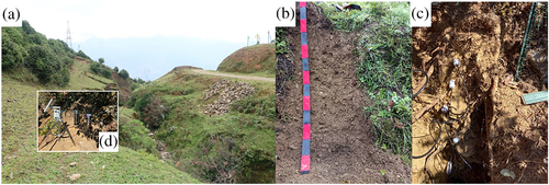
In addition, monitoring of precipitation was carried out in a small valley in XC and the soil moisture was measured (Figure 5). In root zones, soil moisture was measured at depths of 10–90 cm; on slopes (vegetated or bare), moisture was measured only for the upper layer (~20 cm). Coupling moisture and grain distribution prove to be heuristic for understanding the root–soil–water interactions.
3.2 Granular parameters of soil
3.2.1 Graphic parameters
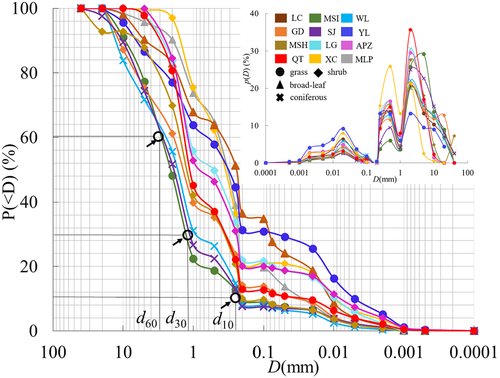
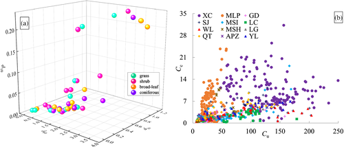
Soils from the test spots are all of multimodal gradation, with frequency peaks at silt (~0.02 mm), fine sand (~0.1 mm), medium sand (~0.5 mm), and coarse sand (~2.0 mm) (Figure 6). Obviously, probability distributions (e.g., Weibull and log-normal distribution) suited to unimodal soils (e.g., Kondolf & Adhikari, 2000; Zobeck et al., 1999) do not fit multimodal cases in general. Instead, various graphic parameters have been employed (e.g., Folk, 1966) to describe the textures—for example, the special grain sizes Dx (e.g., D10, D30, D60) and the coefficient of uniform (Cu) and curvature (Cc), derived from the cumulative curve. These parameters form a scattering dataset (Figure 7); but none is qualified as a synthetic index, and there is no standard method for the descriptions. Furthermore, such a set of parameters cannot take the role as physical variables. Therefore, an integrated index is needed; and the scaling GSD function (Equation 1) has provided the desired parameters μ and Dc.
3.2.2 Scaling GSD parameters
Applying the GSD function (Equation 1) to the soils, we find that all the soils fall into a single exponential curve, P*(D) = exp (−D*) in rescaled coordinates (Figure 8).
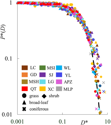
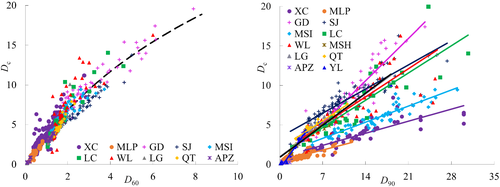
From Figure 8 one sees that the fraction drops rapidly at D > Dc, meaning that most grains (about 85%) are below Dc, so Dc is a characteristic size representing the coarse grains. Consider two representative sizes: D60 and D90. We see that Dc increases with D60 in a logarithmic curve, whereas it increases with D90 linearly (Figure 9). Moreover, D60 is concentrated around Dc, suggesting it is indiscriminate among the soils. On the other hand, D90 differs greatly from one another group of soil, representing the fact that various soils have their own grain size range. Actually, Dc defines the range in that it increases with the upper limit of grain size in a certain curve (Li et al., 2017). At present we do not need to distinguish the sizes, but it suffices to note that Dc represents the coarse textures. In addition, since the soils cover a much wider range (Figure 5) than the USDA triangle of texture (<2 mm), Dc is practically desired for wide-ranging soils. As for the exponent μ, it increases clearly with P(<D) (Figure 10), and thus represents the fraction of relatively fine grains.
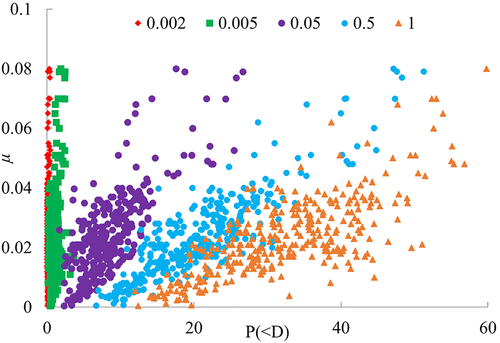
Thus the GSD function provides parameters Dc and μ, respectively representing the coarse and fine textures. Because soil properties depend mainly on fine grains (e.g., Hatheway, 1996), μ is rightly commissioned as the indicative exponent. In the following, we use μ as the synthetic index for soil variability.
3.2.3 Spatial variability of the GSD exponent
- μ Variation in bare soils
- μ Variation in rooted soils
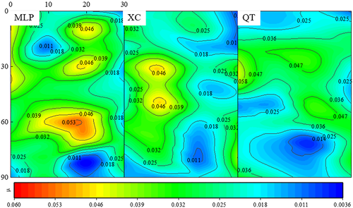
In root zones, the μ-division patterns become complex and vary with roots of different plants (i.e., grass, shrub, broad-leaf and coniferous), as shown in Figure 11, where the soils are of the same types as the bare soils, also sampled from XC and MLP.
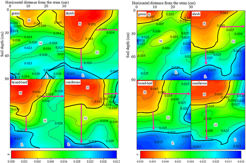
Contrast between μ-division patterns of bare and rooted soil strongly suggests the effect of root on soil texture. The remarkable high-μ-divisions near the roots (Figure 12) imply that the fine grains are highly concentrated there, and this can be traced to the soil–root interaction.
3.3 μ-Division and soil–root interaction
3.3.1 μ-Division responding to root system
Generally, the root system significantly increases matric suction and changes the total head profile, which leads fine grains migrating along with the root water uptake (RWU) (Doussan et al., 2003), forming a coating of clay grains around the root. The effect depends strongly on the abundance of root hairs (Pagès et al., 2000), so that woody plants with deep roots have a strong effect while herbaceous species with shallow roots are weak in RWU (Ehleringer, 2001; Gibbens & Lenz, 2001). These are well shown by the μ-division patterns in different rooted soils.
Now we consider the areas of μ-division in the rooted soils (Figure 12). The area comprises levels of high (H), middle (M), and low (L), with areas AH, AM, and AL, respectively (Table 2), which can be taken as a quantitative index for soil–root interaction. In grass root (herringbone), only a small AH occurs near the surface, because of the short root and weak RWU; while in the others, AH is considerably larger near the root, because of the intense actions of roots (heart-shaped root of shrub and broad-leaf, and taproot of coniferous plant). The difference in μ-divisions between XC and MLP responds to the fact that although soils in XC bear a higher fraction of fine grain, MLP with a high potential of broad and coniferous leaf roots have built a high fraction of AH and AM. It is noted that soils in the shrub regions are similar in the two places, suggesting that shrub roots are randomly distributed on slopes. These findings provide a rough evaluation of RWU. In reality, the total volume (or quantity) of the root system and the growth stage also tip the scales (Zhang et al., 2021). Experiments incorporating filtration and grain migration are expected to reveal the correlation between root–soil interaction and grain distribution.
| μ-Division (%) | Grass | Shrub | Broad-leaf | Coniferous | ||||
|---|---|---|---|---|---|---|---|---|
| XC | MLP | XC | MLP | XC | MLP | XC | MLP | |
| AH | 21.67 | 7.50 | 49.17 | 48.33 | 32.50 | 38.23 | 48.33 | 36.33 |
| AM | 71.66 | 5.00 | 20.00 | 20.00 | 16.33 | 43.25 | 10.83 | 38.67 |
| AL | 6.67 | 87.50 | 30.83 | 31.67 | 51.17 | 18.52 | 40.83 | 25.00 |
3.3.2 Soil–root interaction and RWU
| Site | Gradient direction | ∇μ (%/cm) | ||
|---|---|---|---|---|
| Shrub | Broad-leaf | Coniferous | ||
| XC | H-direction | 4.76 | 5.71 | 7.99 |
| V-direction | 2.14 | 2.86 | 1.22 | |
| MLP | H-direction | 2.33 | 3.35 | 7.59 |
| V-direction | 2.38 | 2.46 | 1.04 | |
Despite vegetation differences in XC and MLP, one observes similar features of ∇μ. In the H direction, both roots of broad-leaf and coniferous plants have higher potential than shrubs; while in the V direction, the remarkably low potential occurs in coniferous roots. This implies that the uptake action is different in the two directions. The H direction is controlled by root uptake while the V direction is dominated by gravity. Therefore, ∇μ can be considered indicative for the potential of root “sucking” fine grains.It is helpful to compare μ-division with moisture pattern, both being correlated with RWU. Figure 13 shows moisture patterns for four types of roots (grass, shrub, broad-leaf and coniferous). One sees that, excepting grass root of weak uptake, the others take a high moisture region near the root. This agrees well with the route of fine grain migration.
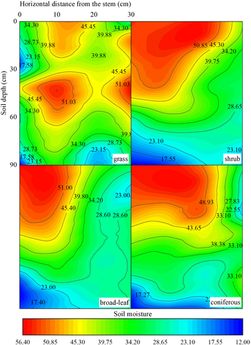
A route map of grain migration can be suggested (Figure 14). The area of root uptake zone has been found to be greatly influential on the moisture profiles (Cassiani et al., 2015); a quantitative correlation, then, should exist between the μ-division and moisture. For grass, the root is 108 cm2, and the high-μ area A (μ > 0.045) covers 18% of the root zone. For the shrub and broad-leaf case, the root system has a similar heart shape, resulting in A (μ > 0.045) of 48%. For the coniferous root zone, the μ-division is impacted hugely by the taproot.
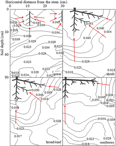
Seepage-induced migration of fine grains in soil (i.e., internal erosion) has long attracted attention in geotechnical engineering (Abdelhamid & EI Shamy, 2015; Kenney & Lau, 1985), but the effect on granular configuration is not quantitatively described in general, except in some numerical simulations (e.g., Cheng et al., 2018). The μ-field provides an intuitive picture of fine-grain migration in response to soil–root interaction. This again confirms the advantage of the GSD parameter.
Considering that the patterns above represent only soils in zones of single root, we go further in applying the method to slopes covered by various plants, expecting that the spatial patterns in rooted soil will occur in areas of large scale.
3.4 μ-Division of soils in vegetated slopes
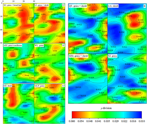
We consider now the surface layer of soil (~20 cm in depth) in the test spots (of size 30 cm × 90 cm). Due to the mixture of roots, the μ-division patterns become more complex (Figure 15), and the division areas and fractions are listed in Table 4.
| Group | Location | μ-Division (cm2) | Area percentage (%) | Mean μ-value | ||||||
|---|---|---|---|---|---|---|---|---|---|---|
| AH | AM | AL | AH | AM | AL | AH | AM | AL | ||
| Blue | QT | 390 | 960 | 450 | 21.67 | 53.33 | 25.00 | 0.054 | 0.030 | 0.017 |
| LG | 285 | 1200 | 315 | 15.83 | 66.67 | 17.50 | 0.056 | 0.028 | 0.016 | |
| MSI | 270 | 1050 | 480 | 15.00 | 58.33 | 26.67 | 0.055 | 0.030 | 0.018 | |
| SJ | 84 | 726 | 990 | 4.67 | 40.33 | 55.00 | 0.053 | 0.033 | 0.017 | |
| Orange | XC | 1350 | 345 | 105 | 75.00 | 19.17 | 5.83 | 0.054 | 0.039 | 0.020 |
| MLP | 600 | 1020 | 180 | 33.33 | 56.67 | 10.00 | 0.052 | 0.034 | 0.017 | |
| GD | 540 | 840 | 420 | 30.00 | 46.67 | 23.33 | 0.056 | 0.033 | 0.018 | |
| LC | 1440 | 240 | 120 | 80.00 | 13.33 | 6.67 | 0.052 | 0.037 | 0.019 | |
| WL | 600 | 1150 | 50 | 33.33 | 63.89 | 2.78 | 0.050 | 0.035 | 0.021 | |
| APZ | 330 | 1380 | 90 | 18.33 | 76.67 | 5.00 | 0.052 | 0.031 | 0.018 | |
- The high-μ group, with remarkable large portion of regions of high μ value, including slopes from XC, MLP, GD, LC, WL, APZ, for which three subgroups can be identified: A1 (XC, LC), A2 (APZ, WL), and A3 (GD, MLP).
- The low-μ group, with remarkable large portion of regions of low μ value, including slopes from QT, LG, MSI and SJ.
In the low-μ group, the slopes are covered by dense grasses and separate shrubs, and the low concentration of fine grain (or small high-μ area) is mainly due to the weak action of shrub and grass roots. On the other hand, the high-μ group is associated with intense root actions. In subgroup A1 (XC and LC), the high-μ regions are connected, owing to the high coverage ratio (76% in XC and 69% in LC) with dense distribution of roots. In subgroup A2 (APZ and WL), the high-μ regions are separated, responding to the moderate coverage ratio (43% in APZ and 45% in WL). Subgroup A3 (GD, MLP) is characterized by a combination of high- and low-μ divisions, because of the low coverage ratio of brush and grass (32% in GD and 29% in MLP).
Again, one sees that the μ-division visualizes the soil variability under interactions between various soils and roots; the patterns in vegetated slopes are the combination of patterns in single-rooted soil where the high-μ region occurs near the root. It is expected that quantitative relationships might be established between the μ-divisions and the root systems when enough data in test spots are available.
4 GRANULAR FIELD OF SOIL
4.1 Probability distribution of GSD parameter
The μ-division above is limited to small test spots; it is practically important, for various hydro-geophysical processes, to build the spatial variability on a large scale (e.g., Chahine, 1992). In previous studies, spatial variability is realized through sampling at test fields over a large area or using the remote sensing data (e.g., for soil moisture) (Brocca et al., 2010). This method is only practicable through time-costing sampling preparations for specific areas but does not formulate a standard routine and operational algorithm. As GSD parameters are random in a soil, we can now extrapolate the μ-variation to large areas based on the probability distribution.
The function curves for the soils are shown in Figure 16 (in which the broken lines denote the data point and the dense curves are the fitted Weibull distribution function), falling into two groups—A (MLP, WL, GD, APZ, LC, XC) and B (QT, LG, MSI, SJ)—just corresponding to the low-μ and high-μ groups in Figure 15. The parameter couple (α, β) determines the curve for each test spot, which represents the total character of granular texture of the soil group.
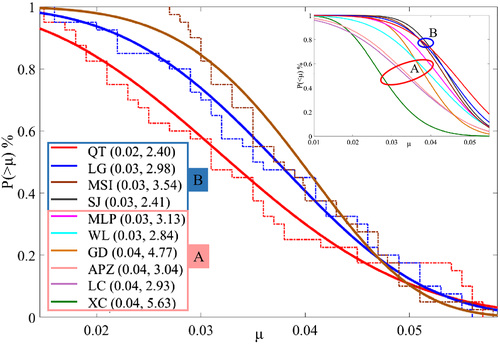
As GSD parameters are random in soil space, the probability distribution is expected to hold on a large scale. Therefore, in principle one may randomly assign μ for each point (or grid cell) of the slope based on the Weibull parameters.
4.2 Establishing a granular field of soil of vegetated slopes
4.2.1 Creating the granular field
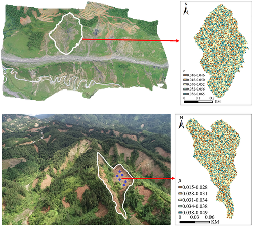
Now we apply the μ-division to the slope scale, based on the probability distribution. We take two slopes in XC and MLP, respectively representing potential landslide and shallow failures, with different soil types and vegetation covers. The test areas of the two slopes are 0.12 km2 and 1163 m2, depending on the landform and surface features. As mentioned above, we have obtained DEM using UAV at a resolution of 0.7 × 0.7 m. Then we randomly assign each cell (at a size of 0.7 × 0.7 m) a value of μ generated by the Weibull distribution, Weib(0.043, 5.63) for XC and Weib(0.029, 3.13) for MLP (cf. Figure 16), and thus create the granular field map of the test slopes (Figure 17). Now the DEM has been assigned a new attribute, the granular character, by the GSD index μ, and it is possible to perform spatial data analysis as one does for geomorphic attributes using the ArcGIS tools. In the following we give two examples.
4.2.2 Implication of granular field
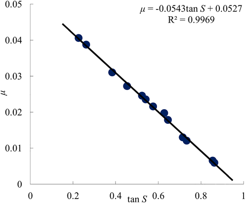
In order to understand how the μ-field is applicable, we consider its relationships to morphology and hydraulic properties. For the morphology factor, we consider the slope gradient, which is crucial for slope stability. We randomly take 12 grid cells on the XC slope and find that the average μ decreases linearly with the gradient, μ = −0.054 tan S + 0.053 (Figure 18), implying that fine grains are inclined to concentrate on gentle slopes. Similar phenomena are also observed in bare slopes, such as the colluvium slopes in mountainous watersheds in southwest China.
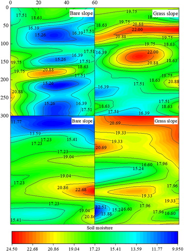
For the hydraulic factor, we consider the moisture (θv) distribution over the slopes in MLP. Randomly measuring moisture at 300 spots of bare and grass slopes (Figure 19, with sites indicated in Figure 17), we find a contrasting trend in bare and grass slopes. In bare slope, θv ~ exp(kB μ), while in grass slope, θv ~ exp(−kG μ). More interesting is that, when Dc-field (i.e., the coarse counterpart of μ-field) is considered, it appears that θ v ~ Dc−n in bare slope and θ v ~ Dc m in grass slope (Figure 20).
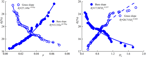
One thing should be noted here, however. The θv-(μ, Dc) relationships, or generally the X-GSD relationships (X being representative soil properties), do not really represent the dynamical causality, but only show a possible state of parameters; because the measurements are randomly taken in space under arbitrary conditions, not in real dynamical processes of a given soil body. At present, the observations merely make sense in that high moisture might occur where the fine grains are clustered or dispersed in bare or grass slopes. Dynamically, the region of high moisture is the sink of RWU and the source of fine grains. One cannot measure moisture without changing the granular texture. Nevertheless, the granular field has revealed the spatial correlations between parameters. It seems that fine and coarse grains are in competitive action in hydraulic processes. Fine content promotes moisture in bare slope and impedes moisture in grass slope, while coarse grains act the other way round.
Moreover, it is possible to establish fields for other parameters derived from the GSD field, through the pedotransfer functions X = f (μ, Dc), and this will be superior to the conventional methods based on measurements of individual samples.
5 DISCUSSION
Hydro-geophysical surface processes strongly depend on soil heterogeneities at all scales; for example, the hydrologic cycle involves calculating fluxes from soil moisture on scales from microscale (~1 km2) to large grid size (~104 km2) (Chahine, 1992), while soil erosion, slope failure, and landslides are governed by spatial variability on the slope scale (~1000 m2) or even soil element scale (~1 m2). In previous studies, the spatial heterogeneity of soil is distinguished by variance of some properties, which are “secondary” variables, each representing one special aspect of soil. In this study the soil heterogeneity is represented by a synthetic granular index derived from a unified GSD function, which is the very “first” variable of soil and plays a fundamental role in determining soil properties, because hydraulic and mechanical properties can be related to the μ and Dc in certain functions (e.g., Gou et al., 2015). This will be helpful in realizing the ambition of deriving soil properties from fundamental and easily measured parameters (e.g., Gupta & Larson, 1979).
The significance of this study lies in the fact that it formulates a method to generate a data space of soil coupled with a specific probability distribution. Compared with the category division of soil properties at large scale, this method is able to create a data space for grid cells at any scale, depending only on data purposes and DEM precision. In addition, the random fields for other soil properties (e.g., Ks, c, and φ) may be easily derived from the granular μ-field through general pedotransfer functions f(μ).
Soil–root interactions have been intensively studied in the context of plant growth and soil genesis (e.g., Glinski & Lipiec, 1990; Gregory, 2006). The μ-division and its spatial pattern similar to moisture distribution suggest that the hydraulic process should be accompanied by a physical process of grain migration, and thus can be well described in term of the GSD parameters. For example, the gradient of μ-field might take a role in the Richards equation. This requires further experimental simulation and field measurements.
A great difficulty in soil science is that one can never measure soil properties without changing the granular texture and structure (hence the GSD). The GSD function is especially favorable in this respect because it preserves the merit of invariance in that the soils undergoing dynamical changes always retain the same GSD function. The variation of GSD parameters does not describe only the spatial variability of soil but also the changes in surface processes.
6 CONCLUSIONS
This study proposes a probability-based method for establishing a random field describing spatial variability of vegetated soils. Compared with previous studies based on field measurements, this method is advantageous in being based on a unified GSD function and using a single synthetic index of granular characteristics.
Under the GSD framework, the spatial variability of soil can be described by a parameter pair (μ, Dc) varying in space. The spatial distribution of μ (the μ-division pattern) intuitively visualizes the fine-grain concentration in soil, and the μ-gradient, coupled to the moisture distribution in soil, quantitatively provides a potential dynamic variable for root–soil–water interaction. Moreover, the GSD parameters in a soil body satisfy the Weibull distribution of probability; this provides the basis for building a granular field on a large scale. The μ-field can be further coupled with other fields of soil properties (e.g., hydrological and mechanical properties) and DEM attributes to form a complete dataset of soil as the base for exploring the related processes and slope stability. In addition, as soil properties can be expressed by pedotransfer functions of the GSD parameters, random fields for fundamental soil properties (e.g., hydraulic or mechanic properties) can be derived from the granular μ- or Dc-field.
Since soil as a system of spatial heterogeneity is representative for earth sciences, the paradigm developed in this study, finding a quantitative description in terms of a synthetic index, is expected to be universally heuristic in formulating theories in a broad variety of fields.
ACKNOWLEDGMENTS
This study is supported by the Strategic Priority Research Program of the Chinese Academy of Sciences (Grant No. XDA23090202), the National Natural Science Foundation of China (Grant No. 41790432, 41977257), and the Key Science and Technology Projects of Transportation Industry (2021-MS4-104).
Open Research
DATA AVAILABILITY STATEMENT
Research data are not shared.


