A simple two-parameter model for scaling hillslope surface runoff
ABSTRACT
The objective of this research was to develop and parameterise a physically justified yet low-parameter model to quantify observed changes in surface runoff ratios with hillslope length. The approach starts with the assumption that a unit of rainfall-excess runoff generated at a point is a fraction β of precipitation P (m) which travels some variable distance down a slope before reinfiltrating, depending on the local rainfall, climate, soils, etc. If this random distance travelled Y is represented by a distribution, then a survival function will describe the probability of this unit of runoff travelling further than some distance x (m). The total amount of per unit width runoff Q (m2) flowing across the lower boundary of a slope of length λ (m) may be considered the sum of all the proportions of the units of rainfall excess runoff integrated from the lower boundary x = 0 to the upper boundary x = λ of the slope. Using these assumptions we derive a model Q(λ) = βPμλ/(μ + λ), (μ > 0, 0 ≤ β ≤ 1, λ ≥ 0) that describes the change in surface runoff with slope length, where μ (m) is the mean of the random variable Y. Dividing both sides of this equation by Pλ yields a simple two-parameter equation for the dimensionless hillslope runoff ratio Qh(λ) = βμ/(μ + λ). The model was parameterised with new rainfall and runoff data collected from three replicates of bounded 2 m wide plots of four different lengths (0.5, 1.0, 2.0 and 4.0 m) for 2 years from a forested SE Australian site, and with 32 slope length–runoff data sets from 12 other published studies undertaken between 1934 and 2010. Using the parameterised model resulted in a Nash and Sutcliffe statistic between observed and predicted runoff ratio (for all data sets combined) of 0.93, compared with –2.1 when the runoff ratio was fixed at the value measured from the shortest plot. Copyright © 2014 John Wiley & Sons, Ltd.
Introduction
The issue of scaling is central to the improvement of hydrologic predictions, encompassing a diversity of hydrologic processes at a large range of spatial and temporal scales (Bloschl and Sivapalan, 1995; Mathier and Roy, 1996; Kirkby, 2001; Cammeraat, 2004; Cerdan et al., 2004; Boix-Fayos et al., 2006). In this paper we focus our attention on the scale dependency of infiltration-excess runoff delivery from slope lengths in the order of 1 to 100 m at the annual-average temporal scale. This spatial scale is of particular practical interest in dissected and undulating terrain where hillslopes with lengths in this range deliver surface runoff and transported pollutants to the drainage network, strongly influencing water quality.
Early plot-scale research concluded that infiltration excess runoff rates per unit width Q (m2) generally increase either linearly or at a decreasing rate with slope length, resulting in rates of runoff per unit area (e.g. mm depth) that are either constant or decreasing with slope-length (Duley and Ackerman, 1934; Wischmeier and Smith, 1965, 1978). Table 1 lists the details of slope length effect studies that have been undertaken since then across a broad range of climates, soil types and land uses. Note the studies of Le Bissonnais et al. (1998) and Palis et al. (1997) are not included in Table 1, as they present data at the storm event scale only.
| Authors | Location | Annual rainfall (mm) | Land condition | Soil description | Slope (degrees) | Plot width/s (m) | Plot lengths (m) |
|---|---|---|---|---|---|---|---|
| Bagarello et al, 2010 (HP) | Sicily, Southern Italy | 700 | Cultivated | Shrink swell clay | 8.5 | 4–8 | 11, 22, 33, 44 |
| Duley and Ackerman (1934) | Kansas, USA | -- | Cultivated | Silty clay loam | c. 2.5 | 1.0 | 3, 6, 12, 30 |
| Bren and Turner (1979) and Bren (1978) | NE Victoria, Australia | 1200 | Eucalyptus forest | Clay loam | 30° | 2.4 | 2.5, 4.8, 12.9, 18.75 |
| Gomi et al. (2008) | South central, Japan | 2000 | Forest | Brown forest soil | c. 40 | 0.5, 8 | ca. 1.5, 25 |
| Joel et al, (2002) | Santiago Chile | 270 | Grazed | Loam | 7.4 | 0.5, 5 | 0.5, 10 |
| Lal (1983) | Western Nigeria, Africa | 900-1300 | Cultivated | Sandy loam Alfisol | 0.6, 2.9, 5.7, 8.5 | 4.0 | 5,10,15,20 |
| Lal (1997) | Ibadan, Nigeria | 1200 | Cultivated | Alfisol | c. 4.6 | 4.0 | 10,20,30,40,50,60 |
| Liu et al. (2000) | Loess Plateau, China | 485–541 | One site fallow, other two cropped | Loess, typical and sandy | 22–30 | 5-15 | 10, 20, 30, 40,60 |
| Moreno-de las Heras et al. (2010) | Central Eastern Spain | 466 | Reclaimed mine slope | Clay loam | 20 | 0.5 | 1,2,3,15 |
| Parsons et al. (2006) | Southern Arizona, USA | ~312* | Desert shrub | -- | 6–10 | 1–11 | 2, 4, 14,19, 28 |
| Sharma (1986) | Jodhpur, India | 360 | Fallow, compacted | Sandy loam loess | 0.3, 2.9, 5.7 | 30–50 | 5,7,8.5,11,14.5 |
| van de Giesen et al. (2000) | Ivory Coast, Africa | 1200 | Fallow, cropped | Loamy sand | 2.3 | 0.8 | 1.25, 12 |
| Xu et al. (2009) | Tibet | 272 | Road side fill slope | Sand and gravel | 30 | 2.0 | 1,2,3,4 |
While most of these studies focus primarily on soil erosion processes, the results all support the slope length–runoff relationship described above. For example, Liu et al. (2000) presented 5 years of runoff plot data from China from lengths varying from 10 to 60 m and found strong negative relationships between the runoff ratio (the ratio of runoff depth to rainfall depth) and slope length for low intensity storms (I30 < 15 mm h-1) and no relationship for higher intensity storms (I30 > 45 mm h-1). Xu et al. (2009) measured runoff from 28 natural rainfall events ranging from 3 to 31 mm from plots 1, 2, 3 and 4 m long on road side-slopes in China. The authors report an inverse power relationship between slope length and runoff per unit area. Bagarello and Ferro (2010) measured runoff from plots in Sicily under natural rainfall varying in length from 0.25 m to 44 m and also reported a statistically significant inverse power relationship in two-thirds of the cases, and non-significant relationships in one-third of cases. Gomi et al. (2008) measured runoff from natural storms in Japan from 2 m and 25 m long plots and report runoff coefficients of 20–40% and 0.1–3%, respectively.
A negative relationship between slope length and per unit area runoff at the hillslope scale is generally attributed to (i) spatial variability in infiltration properties and/or (ii) temporal variability in rainfall intensity. In both cases the result is that surface runoff may be ‘transient’ (Ronan, 1986) and flowpaths ‘discontinuous’ (Gomi et al., 2008). Therefore, runoff that is generated at a point will not necessarily reach the lower boundary of the slope. In the case of spatial variability in infiltration properties, this may occur when surface runoff generated in an area with low infiltration rates is subsequently infiltrated further downslope in an area with high infiltration rates (Nielsen et al., 1973; Brakensiek et al., 1981; Luxmoore, 1981; Sharma, 1986; Watson and Luxmoore, 1986; Williams and Bonnell, 1988; Wilson and Luxmoore, 1988; Loague and Gander, 1990; Price, 1994; Loague and Kyriakidis, 1997; Wilcox et al., 1997; Morbidelli et al., 2006; Jones et al., 2009). Depth-dependent infiltration reported by Langhans et al. (2013) adds additional scaling effects to these spatial effects noted by the above authors. For the case of temporal variability in rainfall intensity, this may occur when the duration of the runoff-producing rainfall event is shorter than the time-of-concentration (i.e. the time it takes for every part of the catchment to be contributing runoff to the outlet) of the hillslope (Stomph et al., 2002; Wainwright and Parsons, 2002; Morbidelli et al., 2006; Reaney et al., 2007).
Spatially distributed dynamic numerical modeling has revealed interesting scaling effects on runoff due to the temporal variability of rainfall (Reaney et al., 2007) and the spatial variability of infiltration (Smith and Hebbert, 1979; Woolhiser et al., 1996; Nahar et al., 2004; Herbst et al., 2006; Morbidelli et al., 2006). Including these numerical models within Monte-Carlo simulations has allowed some researchers to generate mathematical expressions that approximate the scale-effects of spatial variability (Karssenberg, 2006; Morbidelli et al., 2006) and incorporate these into practical runoff and erosion models (Goodrich et al., 2008). Hawkins and Cundy (1987) applied some simplifying assumptions and developed an analytical expression that could set bounds on the effect of spatial variability on runoff generation, an approach that has also proved successful as a practical runoff model (Yu, 1999). Jones et al. (2009) showed analytically that the effect of spatial variability on runoff delivery was well represented using stochastic queue theory, helping to explain mathematically the scaling effects observed in the data and the numerical simulations listed above.
The numerical and analytical approaches described above serve to highlight the complexity involved in representing the spatial and temporal factors that can result in negative relationships between slope length and per unit area runoff at the hillslope scale. The actual relationship between slope length and runoff ratio at a particular location will depend on the interaction between the rate and spatial variability of the soils infiltration capacity and the intensity and temporal variability of the rainfall. As a result, it is currently difficult to scale-up plot scale measurements to the hillslope scale (or vice versa) in a systematic way. For example, in SE Australian forests, Bren and Turner (1979) and Ronan (1986) noted that the interpretation of plot-scale runoff measurements requires caution owing to these kind of scaling effects.
The objective of this research was therefore to develop a simple model (i.e. with few, physically meaningful parameters) to scale runoff ratio estimates at the hillslope scale (c. 1–100 m length), and to determine parameters for this model for a range of landscape conditions.
Model Development
Suppose in the long term a proportion of incoming precipitation reaching the soil surface P (m) becomes infiltration excess runoff at the point scale, and this proportion has the annual average value β (n.d.). That is, if all rainfall-excess generated at the point-scale was instantaneously routed downslope to some lower boundary, summed for the year, then the long-term average of this value would be β. This average proportion would be a function of the local rainfall properties, climate, soils, vegetation, etc.
 (1)
(1) (2)
(2)However, the distribution of Y, fY(y), is as yet unknown. We assume here the random flowpath length Y has a Pareto Type II distribution, also known conditionally as the Lomax distribution. To the knowledge of the authors, there has been no research to measure the flowpath length y under field conditions, therefore the Lomax distribution was chosen based on the following logic. A heavy tailed distribution was preferred because the natural convergence and concentration of runoff on a hillslope would likely result in some small proportion of runoff travelling a very long distance. In addition, infiltration-excess runoff that travels a long distance typically comes from intense rainfall events, and it is known that rainfall intensity has a heavy tailed distribution (Brown and Foster, 1987).
 (3)
(3) (4)
(4) (5)
(5) (6)
(6)The parameter α controls how heavy the tail is of the Lomax density function. Smaller values of α produce a heavier tail, however, α needs to be greater than 1 for Y to have a mean. Ideally α could be fitted, however, it was felt that this was not justified at this time given the limited available data, the limited knowledge of the true distribution of y, and the fact that α is not directly physically interpretable like μ. Fixing the value of α reduces the number of fitting parameters in the model from 3 to 2. The value of α was therefore fixed, and set at a value of 2, as this provides for a simple analytic result from the integration in Equation 2, and results in the Lomax distribution parameter μ representing the mean travel distance of a unit of infiltration excess runoff (Equation 6).
 (7)
(7) (8)
(8)Equation 8 can be recognised as a rectangular hyperbola, the function 1/λ dilated by a factor of βμ and translated μ to the left. The behaviour of Equations 7 and 8 is consistent with physical constraints. When the annual-average point-scale runoff ratio β is zero, hillslope scale runoff is also zero. As the mean travel distance of a unit of rainfall excess μ approaches zero, hillslope scale runoff also approaches zero. As the mean travel distance becomes very large, the hillslope runoff ratio Qh approaches the point scale runoff ratio β. This is approximately equivalent to routing all point-scale runoff directly to the lower boundary. At zero slope-length the hillslope runoff ratio is equal to the point scale runoff ratio β, while the runoff rate is zero. For a given location, total runoff Q increases linearly with precipitation P.
- β = 0.5 and μ = 1 m
- β = 0.5 and μ = 10 m
- β = 0.9 and μ = 10 m
- β = 0.9 and μ = 25 m
- β = 0.9 and μ = 100 m
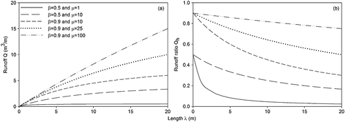
In the first case 50% of rainfall becomes runoff at the point scale, however, this runoff re-infiltrates a short distance (with a mean of 1 m) downslope, resulting in a highly non-linear relationship between slope length and runoff ratio. In the second case, the same proportion of rainfall becomes runoff at the point scale, however, this runoff travels on average 10 m, and the relationship between slope length and runoff ratio therefore becomes more linear. In cases 3–5, the point-scale runoff ratio is 0.9, and comparing these three cases with the previous two illustrates that the β parameter represents the y-intercept in the plot of plot-length against runoff ratio (Figure 1(b)). Cases 3–5 also illustrate the effect of increasing the mean flowpath length μ on the linearity of the relationship between slope-length and the runoff ratio.
Parameterisation Methods
New rainfall-runoff data
A rainfall-runoff study was conducted in north-east Victoria, Australia, to generate data to quantify the β and μ parameters in Equation 8. The study was undertaken in an area adjacent to a tributary of the Long Corner Creek catchment, Flat Creek, referred to as LCCA (Figure 2). A detailed description of the study area is provided in Smith et al. (2010), and a brief description is given here. The catchment supports a mature damp to dry open Eucalyptus forest. The dominant species include narrow-leaved peppermint (Eucalyptus radiata), broad leaved peppermint (E. dives), red stingybark (E. macrorhyncha) and manna gum (E. viminalis). In the lower part of the catchment the understory is dominated by European blackberry (Rubus fruticosus aggregate), particularly in the near stream area. Soils are gradational with silty loams at the surface changing to heavy clay with depth. The closest Bureau of Meteorology weather station is located at Lake Buffalo (station ID 083079 3.4 km south-east of LCC at 36°42′48″ S and 146°40′18″ E) and between 1961 and 1990 the mean annual rainfall measured at this site was 1057 mm with a standard deviation of 247 mm. A fuel reduction burn was conducted in LCC A between 3 and 5 April 2006. Fire was confined to the areas around ignition points and to the near stream area of lower catchment, due to the high fuel moisture levels at the time of burning.
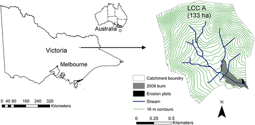
Three replicates of four different length plots 2 m wide and 0.5 m, 1 m, 2 m and 4 m in length (giving 12 plots in total) were constructed within a 100 m x 100 m area on the lower north-east slope at 36°41′S and 146°38′ E (Figure 3) which had recently been burnt by a low intensity fuel reduction burn.

Plot locations were chosen with a slope gradient of 20 (±2) degrees. Plots were bound at the top and sides using pieces of sheet metal that were 200 mm wide and either 550 or 1050 mm in length, allowing the sheets to overlap by 50 mm. Sheets were hammered between 20 and 50 mm into the ground to form the rectangular plot boundary. Sheet metal collection trays were installed on the lower end of the plots. The trays were 2 m wide and 0.75 m deep in the shape of an isosceles triangle, with the side edges folded 90° to the surface to form an 80 mm rim which protruded 50 mm forward of the bottom edge, to form a flange. Pop rivets were used to fasten the overlapping metal plot edges together, and where the plot edges overlapped with the flanges of the collection trays. The front edge of the collection tray which formed the plot end (2 m in wide) was folded down 90° to form a 50 mm lip that was hammered into the ground, and sealed to the natural soil surface using cement. In addition to this lip, the collection trays were also supported by pieces of angle iron hammered into the ground and bolted to each side of the collection tray outlet, allowing the slope of the trays to be adjusted to match the soil surface. Collection trays were covered with a metal lid to stop any rain water entering the collection tank. Water flowed by gravity out of the trays and into individual collection tanks via an 80 mm diameter PVC pipe. Collection tanks were installed on level concrete pads below the collection trays. The tanks had a removable lid and were either 150 or 250 L in capacity, depending on the length of the plot. Rainfall reaching the soil surface P (m) (i.e. the rainfall not intercepted by the forest canopy) was measured using a tipping bucket pluvio with a tip volume of 0.1 mm mounted at a height of 1 m from the ground surface, cross-checked against two manual rainfall gauges above and below the area of the experimental plots, also mounted at the same height.
The site was serviced after rainfall events of 20 mm or more, or at monthly intervals regardless of total rainfall. The first site service was on 11/05/2006 (1 month after the fuel reduction burn) and the last site service was on 01/05/2008, approximately 2 years after the burn. The volume of water that accumulated in the tanks was measured using a ruler and the depth in centimetres was converted to a volume in litres using a calibrated depth–volume conversion chart for the different tank sizes.
An approximate estimate of the percentage of the surface of each plot covered by vegetation and litter was assessed visually during each site visit, using field cover charts (McDonald et al., 1990). During each site visit a soil core 73 mm inside diameter and 57 mm deep was taken from the soil surface adjacent to the plots and the gravimetric water content determined by drying it in an oven at 105 °C for 48 h. In addition, soil water repellence tests were completed on the mineral soil surface in both the burnt and unburnt areas using a simplified version (McDonald et al., 1990) of the molarity of ethanol droplet test. The field method is a simplification of the approach of King (1981) and utilises a comparison of the ability (yes/no) for water and 2 mol L-1 ethanol to penetrate the soil in 10 s. This provides a broad classification of water repellency into three classes: nonwater- repellent, where a water drop infiltrates in ≤10 s; water-repellent (R), where water infiltrates in >10 s and 2 mol L-1 ethanol infiltrates in ≤10 s, and strongly water-repellent, where 2 mol L-1 ethanol infiltrates in >10 s.
Rainfall simulation (RFS) experiments were also conducted at the field sites to quantify infiltration rates under rainfall. A detailed description of the rainfall simulation procedure can be found in Sheridan et al. (2007). Briefly, rainfall was simulated at an energy of 295 kJ ha-1 mm-1 over three 1.5 m wide 2 m long plots in July 2006 and March 2007. The rainfall simulator uses three 80100 VeeJet nozzles spraying downwards and oscillating across the plot area, with an adjustable frequency to achieve the desired intensity. In July 2006 three different intensities were used, 100, 50 and 25 mm h-1 on each plot (with the highest intensity applied first), while in March 2007 only one intensity of 100 mm h-1 was used. The rainfall simulator is a design that was modified by Loch (1989).
Supplementary local rainfall-runoff data
Additional rainfall-runoff data from other local plot scale studies were compiled to extend the range of slope lengths and add to the quantity of data generated from the forested field experimental sites.
Bren (1978) and Bren and Turner (1979) collected runoff over a 7 month period from the Cropper Creek catchment located approximately 12 km SSW of the study area, from two bounded plots that measured 2.5 and 4.8 m in length and 2.4 m wide, with an average slope of between 25 and 30°. The site had an average annual rainfall of 1412 mm (Bren and Hopmans, 2007), and the geology is Ordovician sandstones and shales, with highly porous clay loam soils. The forest type was similar to Long Corner Creek catchment, with narrow-leaf peppermint (E. radiata) being the predominant tree species, and manna gums (E. viminalis) along the streams, brittle gums on the spurs (E. mannifera), and an understory dominated by bracken fern (Pteridium esculentum) (Bren, 1978).
Ronan (1986) collected runoff from four 20 m long and 20 m wide plots with an average slope of 20°, over a 10 year period between 1970 and 1980. Sites were located approximately 40 km NNE from Melbourne Victoria 37°25′ S and 145°10′ E, in a similar damp eucalypt forest with similar soils and climate. Average annual rainfall was 1220 mm and was measured at a site 0.8 km south-west of the experimental plots. The geology is comprised of lower Devonian siltstone, and the soil is a stony clay loam. Vegetation of the study area was classified as a dry mixed species Eucalyptus forest, consisting mainly of broad and narrow leaved peppermint (E. dives and E. radiata), with the occasional messmate (E. oblique) and red stringybark (E. macrorrhyncha), and an understory dominated by bracken fern (Pteridium esculentum). Plots were monitored for 2.5 years before two plots were subjected to a fuel reduction burn. A low intensity fuel reduction burn was applied to another plot after 4.5 years, with one plot remaining unburnt for 8.5 years until a moderate intensity fire swept through the area. A subset of plot data collected from the unburnt plots and the low intensity fuel reduction burn plot were selected for this analysis.
Rainfall-runoff data from the literature
Additional rainfall-runoff data from multi-length plot studies in the international literature were compiled to enable parameters to be determined for a range of landscape conditions. A search of the literature yielded 12 published studies from 1934 to 2010 with 32 data sets from plots of different length that could be used to determine values for the β and μ parameters in Equation 8. The details of these studies are listed in Tables 1 and 4.
New rainfall-runoff data
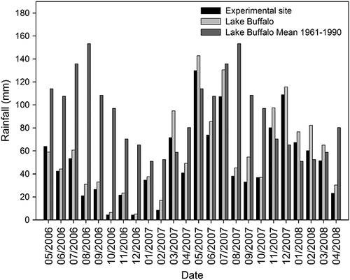
The total rainfall P measured at the experimental site (beneath the forest canopy) over the period April 2006 to May 2008 was 1212 mm; 403 mm in the first year and 809 mm in the second year. Monthly P totals at the experimental site were compared with rainfall totals at Lake Buffalo (3 km to the south-east) for the experimental period, and the long-term (1961–1990) mean rainfall also at Lake Buffalo (Figure 4). This data illustrates that (a) the monthly rainfall at Lake Buffalo and the monthly throughfall at the experimental site are generally highly correlated (R2 = 0.96), and therefore our short-term record at the experimental site can reasonably be compared with the long-term mean at Lake Buffalo, and (b) based on this observation, the first 12 months of the experiment the site received 42% of the average rainfall amount.
The fuel reduction burn consumed all of the surface vegetation in the area of the experimental plots so the vegetation cover at the beginning of the plot runoff measurements was zero. There was very little vegetation recovery in the first year after the fire (c. 10–20%), with consistent recovery in the second year, reaching an asymptote of c. 90% vegetation contact cover at the end of the study. The GWC of the soil varied from c. 27% in winter 2006 to c. 4% in summer 2006–2007. The soil was recorded as non-water repellent during all site service visits for the study period, except for 28/12/2006 and 1/2/2007, when the soil was rated as repellent and severely repellent, respectively, corresponding to the lowest soil GWC for the study period.
The results from the rainfall simulation experiments in July 2006 and March 2007 are given in Table 2. The results showed that the infiltration rate increased strongly with rainfall intensity, from 21, to 40, to 76 mm h-1 at rainfall intensities of 25, 50 and 100 mm h-1, respectively. These results indicate the infiltration capacity of the plots under rainfall had not been reached at 100 mm h-1 rainfall intensity.
| Date | Nominal Intensity (mm h-1) | Actual Intensity (mm h-1) | Runoff rate (mm h-1) | Infiltration rate (mm h-1) | Runoff ratio (%) |
|---|---|---|---|---|---|
| July 2006 | 25 | 23 | 2(2) | 21(2) | 10(7) |
| 50 | 48 | 8(4) | 40(4) | 17(9) | |
| 100 | 95 | 19(9) | 76(10) | 20(10) | |
| March 2007 | 100 | 97 | 17(8) | 80(11) | 18(8) |
Infiltration rates under simulated rainfall remained similar over the 2 years of observation (mean of 76 mm h-1 in the first year, compared with 80 mm h-1 in the second year) suggesting little change in soil hydrologic properties due to low intensity fuel reduction burn at this site. Large differences in annual rainfall during the vegetation recovery period (403 mm in the first year, compared with 809 mm in the second year) were considered likely to obscure any vegetation recovery effects in this study, and the role of low intensity fire is not considered further here. The analysis is split into two water years due to the large annual rainfall differences observed during the study.
The results from each of the replicated runoff plots under natural rainfall are shown in Table 3. It is assumed that all runoff is infiltration-excess runoff because the soils are well drained, and the experimental plots were located on a steep section of hillslope in a position elevated from the gully. Saturation was never observed in the plot area during the experimental period. Table 3 shows that runoff to the plot boundary (L) increased with slope length, but at a decreasing rate. Note that in the first year the total runoff from the 4 m plot was lower than the 2 m plot.
| Plot length (m) | ||||||||
|---|---|---|---|---|---|---|---|---|
| Runoff (L) | 0.5 | 1 | 2 | 4 | ||||
| Year 1 | Year 2 | Year 1 | Year 2 | Year 1 | Year 2 | Year 1 | Year 2 | |
| Rep 1 | 25.8 | 83.8 | 62.9 | 156.7 | 76.7 | 144.8 | 89.8 | 139.6 |
| Rep 2 | 38.7 | 124.6 | 68.9 | 174.5 | 88.2 | 175.1 | 51.0 | 177.2 |
| Rep 3 | 37.4 | 78.2 | 50.6 | 94.4 | 125.7 | 134.1 | 19.3 | 189.9 |
| Mean runoff (L) | 34.0 | 95.5 | 60.8 | 141.9 | 96.8 | 151.3 | 53.4 | 168.9 |
| Mean runoff (mm) | 34.0 | 95.5 | 30.4 | 70.9 | 24.2 | 37.8 | 6.7 | 21.1 |
| Mean runoff to rainfall ratio | 8.4 | 11.8 | 7.5 | 8.8 | 6.0 | 4.7 | 1.7 | 2.6 |
Supplementary local rainfall-runoff data
The new rainfall-runoff data collected from the multi-length runoff plots at LCC A were supplemented with additional data reported by Bren (1978), Bren and Turner (1979) and Ronan (1986). Runoff data collected by Bren (1978) from plots 2.5 and 4.8 m in length produced runoff to rainfall ratios of 6.01 and 3.55, respectively. Applying these runoff to rainfall ratios to the total rainfall depth that occurred during the first and second years at LCC, the runoff at LCC for the two plot lengths was estimated to be 0.06 and 0.12 m3 m-1 width for the 2.5 m plot, and 0.07 and 0.14 m3 m-1 width for the 4.8 m plot for the first and second years, respectively.
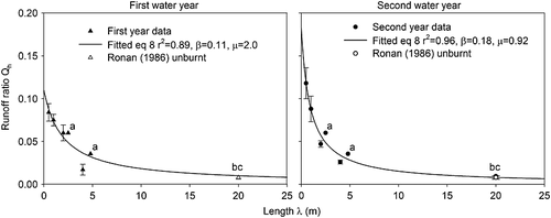
Ronan (1986) collected runoff from plots 20 m long in a similar forest type that was subjected to a low intensity prescribed fire, with similar soil type and climate over a 10 year period. Data collected from plots exposed to a fuel reduction burn were split into two water years to match the treatment applied at LCC. From this data a runoff ratio of 0.77 and 0.94% was calculated for the first and second years (after burning), respectively. Following the same procedure above, the total runoff at LCC for a 20 m plot was estimated to be 0.06 and 0.15 m3 m-1 width for the first and second years (Figure 5). In addition to these data points but not used in the fitting of the function, the average runoff rainfall ratio for the unburnt plot data from Ronan (1986) was calculated to be 0.79%. Data were available from four replicated plots and this enabled the calculation of error bars. Using this approach a total runoff of 0.06 and 0.13 m3 m-1 width was estimated for the first and second years, respectively.
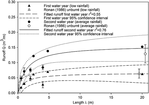
Figure 6 plots the data from Figure 5 as runoff ratios, and the curves show the fit of Equation 8 to this data.
Rainfall–runoff data from the literature
In Figure 6, Equation 8 is shown fitted to the new data from this study, Ronan (1986) and Bren (1978), for the first and second year of the study to determine the values of the point-scale runoff ratio β (nd) and the mean runoff length μ (m). A search of the literature provided a number of runoff data sets from plots of different length that could also be used to determine the value of β and μ. The details of these studies, along with the goodness of fit of Equation 8 and the value and significance of the β and μ parameters are summarised in Table 4. Note that in the fitting procedure the value of β is constrained to 0 ≤ β ≤ 1 and the value of μ is constrained to μ >0. The fitted models and the literature data are illustrated in Figure 7. Within some studies plot treatments were similar at different sites, therefore the average runoff ratio was used in the fitting of Equation 8, where this occurred both individual and average site results are presented in Table 4.
| Data source | Β | μ | R2 | N | Treatment | Details of data used in fitting | ||
|---|---|---|---|---|---|---|---|---|
| Value | p | Value | p | |||||
| This study | Forested | Described in methods section of this paper | ||||||
| Dry year | 0.11 | 0.002 | 2.00 | 0.066 | 0.89 | 8 | ||
| Wet year | 0.18 | 0.001 | 0.92 | 0.020 | 0.96 | 8 | ||
| Bagarello et al. (2010) | 0.42 | 0.092 | 8.71 | 0.234 | 0.86 | 6 | Cultivated fallow | Mean runoff ratio from Table 2 |
| Duley and Ackerman (1934) | 0.39 | 0.010 | 34.33 | 0.154 | 0.84 | 4 | Cultivated | Runoff from natural rainfall events from Table 1 |
| Gomi et al. (2008) | Forested | Plot lengths from Table 1, data from Results section. ‘Rainfall and Runoff in Small and Large Plots’ | ||||||
| Site 1 | 0.30 | 13.09 | 2 | Cypress plantation, sparse understory | ||||
| Site 2 | 0.32 | 2.05 | 2 | Hinoki plantation, dense understory | ||||
| Site 3 | 0.73 | 0.25 | 2 | Deciduous forest, dense understory | ||||
| Joel et al. (2002) | Pasture | Total rainfall from Table 2, total runoff from Table 3 | ||||||
| Site 1 | 0.43 | 3.58 | 2 | |||||
| Site 2 | 0.49 | 5.15 | 2 | |||||
| Site 3 | 0.33 | 9.81 | 2 | |||||
| Average | 0.41 | 5.59 | 2 | |||||
| Lal (1983) | Cultivated | Total rainfall from Table 2, total runoff from Table 4 | ||||||
| Plots 1,2,3,4 | 0.18 | 0.206 | 65.00 | 0.795 | 0.08 | 4 | Slope 1% | |
| Plots 5,6,7,8 | 0.91 | 0.080 | 4.22 | 0.166 | 0.96 | 4 | Slope 5% | |
| Plots 9,10,11,12 | 0.81 | 0.114 | 4.90 | 0.239 | 0.92 | 4 | Slope 10% | |
| Plots 13,14,15,16 | 0.50 | 0.081 | 8.36 | 0.235 | 0.88 | 4 | Slope 15% | |
| Lal (1997) | Cropped | Rainfall and runoff from Table 2 | ||||||
| 0.113 | 0.014 | 154.50 | 0.494 | 0.17 | 6 | Convention al till | ||
| 0.088 | 0.034 | 16.02 | 0.139 | 0.90 | 5 | No till | ||
| Liu et al. (2000) | Cropped | Mean annual runoff from Table 2, mean annual rainfall pers. comm. | ||||||
| Ansai site | 0.10 | 0.003 | 130.12 | 0.099 | 0.85 | 4 | Fallow | |
| Suide site | 0.05 | 0.059 | 112.48 | 0.247 | 0.91 | 3 | Tilled and cropped | |
| Zizhou site | - | - | - | - | Tilled and cropped | |||
| Moreno-de las Heras et al. (2010) | Disturbed | Total rainfall from Table 2, total runoff from Table 3 | ||||||
| Slope 1 | 0.27 | 0.007 | 48.50 | 0.338 | 0.53 | 4 | Rilled, <10% vegetation cover | |
| Slope 2 | 0.24 | 0.005 | 84.36 | 0.436 | 0.36 | 4 | Rilled, <10% vegetation cover | |
| Average Slope 1 and 2 | 0.26 | 0.006 | 61.73 | 0.376 | 0.46 | 4 | ||
| Slope 3 | 0.21 | 0.013 | 39.09 | 0.397 | 0.46 | 4 | Transitional | |
| Slope 4 | 0.34 | 0.403 | 1.32 | 0.629 | 0.41 | 4 | Poor rills, 45-60% veg cover | |
| Slope 5 | 1.00 | 0.725 | 0.24 | 0.767 | 0.88 | 4 | No rills, 45-60% veg cover | |
| Parsons et al. (2006) | 0.40 | 0.006 | 22.34 | 0.14 | 0.78 | 5 | Forested Desert shrub | Mean runoff coefficients estimated from Figure 5 |
| Sharma (1986) | 0.57 | 0.003 | 12.64 | 0.043 | 0.92 | 5 | Fallow, Compacted first year of 7 | Mean annual runoff ratio from Table 3 |
| van de Giesen et al. (2000) | Cropped | Runoff data from Table 1 | ||||||
| Plot 1 | 0.41 | 12.79 | 2 | Bare fallow/rice | ||||
| Plot 2 | 0.50 | 14.16 | 2 | Bare fallow/rice | ||||
| Average plots 1 and 2 | 0.45 | 13.49 | 2 | |||||
| Plot 3 | 0.56 | 1.39 | Weedy fallow/rice | |||||
| Xu et al. (2009) | 1.00 | 0.185 | 0.78 | 0.321 | 0.93 | 4 | Disturbed Bare road side-slopes | Mean runoff ratio from results section and Figure 2 |
- N: number of slope length plots in the study.
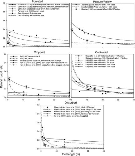
The value of β varied from a minimum of 0.05 for a cropping site on the Loess Plateau in China (Liu et al., 2000) through to a maximum of 1.00 (P = 0.725) for roadside fill-slopes (P = 0.185) (Xu et al., 2009) and reclaimed mining slopes (P = 0.725) (Moreno-de las Heras et al., 2010). It is important to note that these maximum β have high P values and should be treated with caution. A value of β = 1 is physically unrealistic for an infiltrating soil, and these unrealistically high values are probably an artefact of the limited spread of the data for these studies and the fitting procedure. The maximum significant (P < 0.05) β value was 0.57 (P = 0.003) for a fallow compacted sandy loam loess from India (Sharma, 1986). The value of the mean runoff length μ varied over three orders of magnitude from a minimum of 0.24 (P = 0.767) for a reclaimed mining slope in the Mediterranean (mean rainfall 466 mm yr-1) (Moreno-de las Heras et al., 2010), through to a maximum of 154.50 (P = 0.494) for cultivated soils in Nigeria (Lal, 1997). This large variability in μ highlights the highly variable and often strongly non-linear effect of slope length on the runoff ratio.
Inspection of the curves fitted in Figure 7 and the site-based attributes listed in Table 1 and Table 4 indicates that there is no clear systematic relationship between physiographic variables and the fitted values of the β and μ parameters. Despite this, some qualitative patterns do deserve mention. Figure 7 groups the experimental data set into land-use types (forested, cultivated, etc.). From observation there are no large systematic differences in the kinds of slope length responses as a function of land-use type. Within each land-use type there is an equally wide range of responses. The study of Lal (1983) indicates that slope angle can have an effect on μ, with flat slopes showing no effect of slope length (μ = 65) on the runoff ratio, while steeper slopes illustrate a stronger non-linear response (μ = 8.36) to slope length. However, the data from Liu et al. (2000) is from very steep sloping plots and shows no effect of slope length (e.g. μ = 130.12 for the fallow site).
The sites with the lowest μ values were observed to be strongly affected by rilling. The plots of Moreno-de las Heras et al. (2010) cover a spectrum of sites from bare and rilled, to vegetated and unrilled. The runoff ratio from the rilled plots shows a relatively linear relationship with slope length (μ > 40) while those with the least rills are strongly non-linear (μ = 0.24). This may be due to a high level of connectivity within the rilled plots, resulting in rapid time of concentration during storms. The undisturbed forested sites with high rainfall, Gomi et al. (2008) and this study, show high non-linearity (0.25 ≤ μ ≤ 13.09).
Model calibration
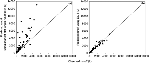
Using the data from the studies listed in Table 4 (except for Duley and Ackerman, 1934) we compare the use of the runoff ratio measured from the shortest plot (i.e. assuming no scaling effect) to the use of Equation 8 with the calculated β and μ coefficients listed in Table 4 to predict runoff from each of the larger plots in each study. These predictions were compared with the observed runoff rates from each of the larger plots from each study (Figure 8). The Nash and Sutcliffe (1970) statistic was used to compare the predicted and observed values in each case. Using the runoff ratio measured on the shortest plot to predict the runoff ratio of the largest plot yields a Nash and Sutcliffe (1970) statistic of –2.1, while using Equation 8 yields a statistic of 0.93. An efficiency of 1 corresponds to a perfect match of modelled values to the observed data. An efficiency of 0 indicates that the model predictions are as accurate as the mean of the observed data, whereas an efficiency less than zero occurs when the observed mean is a better predictor than the model. Note that this analysis uses all the data that was used to fit Equation 8, and is therefore a measure of the quality of the calibration of the model, rather than a test of its predictive capacity. Nonetheless, this analysis does illustrate that the model is of a suitable form for scaling runoff ratios under a broad range of site and climatic conditions.
Discussion
Model assumptions
When applying Equation 8 careful consideration should be given to the conditions under which the expression remains valid. If the function is calibrated using empirical runoff data, then it is assumed that the experimental plots are representative of the soil and site conditions at the spatial scale of the model predictions. It is also important to consider the likelihood of a change in hydrologic process across the range of scales under investigation to ensure that the dominant processes at the scale of model parameterisation are also dominant at the scale of model prediction (Cammeraat, 2004).
It also should be noted that the observed non-linear increase in runoff with slope length is generally attributed to both spatial and temporal properties of the system. However, temporal effects are only likely to be observed if the duration of runoff generating rainfall events is short relative to the time of concentration for the slope length of interest. It is likely therefore that the data collected from short plot lengths, such as the field plots in this study (0.5–4 m), do not incorporate all of the temporal effects noted above, which may result in an even greater non-linearity between slope length and runoff ratio. Several authors (Julien and Moglen 1990; Van de Giesen et al., 2000, 2005, 2011; Wainwright and Parsons, 2002) have explored the relative roles of spatial versus temporal system properties in relation to the scaling of runoff ratios, however, the annual-scale data sets presented here do not provide insight into these causal processes of runoff scaling.
The parameters fitted to Equation 8 are a function of the rainfall and soil conditions over the period of data collection. Applying the model with the fitted parameters to other time periods should be undertaken with consideration of the potential differences in conditions between the model calibration and the model application period. The model is based on infiltration-excess runoff processes and does not attempt to capture the effects of slope length on saturation excess runoff processes, which has been explored by Aryal et al. (2003). The model is not applicable to conditions of saturation in its current form.
The model assumes a Lomax distribution for the random flowpath length Y with an α parameter set to the value 2. If future research reveals better choices for the distribution of fY(y) and/or the value of α, then Equation 3 should be replaced with a more suitable density function, and the integrations in Equation 1 and 2 recalculated. This would likely result in different models in Equation 7 and 8, and possibly different parameters. It is possible that the data sets listed in Table 4 which were poorly fitted to the model, such as the Lal (1983) low slope data (R2 = 0.08), would be better represented with a different distribution for Y.
Determining model parameters
The parameters β and μ are likely a function of the complex interaction between the temporal variability of precipitation and the spatial variability of the infiltration capacity of the soil for the period of observation. As such, both β and μ should be considered as long-term averages for point scale runoff ratio and flow length, respectively. These ‘system parameters’, should be interpreted conceptually in a similar way to how runoff ratios are currently interpreted.
Parameters for Equation 8 can be determined by measuring rainfall and runoff rates from plots of at least two different lengths and fitting the equation to the data using a least squares approach. Ideally, the longest plot should be of sufficient length to capture the effects of temporal variability in rainfall. The optimal maximum length will depend on the time of concentration of runoff on the plot, and the duration of storm events. Rainfall and runoff data should be collected for a period of time sufficient to capture the natural variability in rainfall and soil conditions at the site of interest. In the absence of field plot data, interpretation of the parameter results in Table 4 may enable a first approximation of the likely value of these parameters based on similarity to the sites (listed in more detail in Table 1) for which parameters have been determined in this study. A more detailed analysis of these plot-length data sets in the literature may reveal predictive relationships between the parameters β and μ and local properties that may be expected to influence infiltration excess runoff scaling, such as rainfall, soil, slope and vegetation properties, enabling the model parameters to potentially be estimated from available spatial data.
It is also possible that the parameters β and μ, which have clear physical interpretations, could be measured directly in the field. For example, point-scale runoff measurement devices such as runoff cups, or difference infiltrometers (Moody and Ebel, 2012), could be used to estimate the β parameter. The travel distance of overland flow could possibly be estimated using fine sediment tracers. The capacity for directly measuring these model parameters and using them to predict the observed variability in scale effects is an area for future research.
Model applications
The most obvious application of Equation 8 is to better estimate runoff from hillslopes of different lengths λ. The results shown in Figure 8 illustrate that this can make a large difference to the estimate of runoff, especially when the value of the flowpath length parameter μ is small. Bagarello et al. (2013) showed the importance of incorporating information on the slope–length dependence of the runoff ratio for correctly estimating hillslope erosion rates using the USLE-MM model. Equation 8 provides a physically justified yet low parameter method to represent this dependence.
 (9)
(9)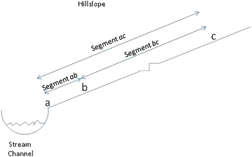
So, for example, for the second year at the experimental site β = 0.18 and, μ = 0.92 which means that in this catchment for a 100 m long hillslope 85% of the runoff is sourced from within 5 m of the lower boundary of the slope.
Summary
A negative relationship between slope length and the runoff ratio at the hillslope scale (c. 1–00 m slope length) has been commonly observed. The objective of this research was to develop and parameterise a physically justified yet low-parameter model to quantify this observed scale-dependency of the runoff ratio. The model assumes that, on average, for a given site, some characteristic proportion of rainfall β becomes runoff at the point scale. This runoff Q then travels some variable distance down a slope (with a mean distance of μ) before re-infiltrating, depending on the local rainfall, climate, soils, etc. Based on these assumptions, a simple two-parameter model of surface runoff as a function of slope length was developed. The parameters β and μ represent the point scale runoff ratio (non-dimensional) and the mean flow path length (m) of a unit of runoff, respectively. The value of these parameters was determined using new data from plot-length experiments on forested hillslopes, combined with existing data from plot-length field studies reported in the literature. The new model was parameterised by fitting to these data, showing that for the range of experimental conditions the point scale runoff ratio parameter β varies from 0.05 to 1.00, while the mean runoff length parameter μ varies from 0.24 to 155 m. Locations with short runoff flow paths (i.e. low values of μ) display a highly non-linear relationship between slope length and runoff ratio.
Both the β and μ parameters can be determined by fitting the model to surface runoff data collected from at least two different plot lengths over a period representative of the long-term average conditions at the site. The parameterised function enables runoff ratios to be estimated for slopes of different length (i.e. allows the runoff ratio to be scaled) and allows the source (i.e. the location along the hillslope) of infiltration excess runoff to be estimated. Future investigations should aim to establish ways to predict the parameter values for the model for broadly different landscape and climate combinations, to allow the application of the model in the absence of field runoff plot data.
Acknowledgements
The authors would like to sincerely thank John Costenaro for his tireless field support. This project was funded by the Department of Sustainability and Environment, Victoria, and the Cooperative Research Centre Forestry. Many thanks to the reviewers of this manuscript, whose suggestions greatly improved the final paper.
Notation
| Symbol | Meaning | Type | Units | Value range |
| P | Precipitation reaching the soil surface | scalar | m | [0, ∞] |
| α | Shape parameter for the Lomax distribution | scalar | non- dimensional | (1,∞] |
| β | Annual average point scale proportion of rainfall excess | scalar (fraction) | non- dimensional | [0,1] |
| μ | The mean travel distance of a unit of rainfall excess | scalar | m | (0, ∞] |
| λ | Hillslope length | scalar | m | [0, ∞] |
| x | Distance above the lower boundary | scalar | m | [0, λ] |
| Y | Random travel distance of a unit of rainfall excess | random variable | m | [0, ∞] |
| y | Travel distance of a unit of rainfall excess | scalar | m | [0, ∞] |


