Lead high-damping rubber (LHDR) bearings, composed of high-damping rubber and lead core, are effective isolation devices that address increased seismic demands. The temperature effect on the behavior of LHDR bearings is significant, leading to increased initial stiffness at low temperatures. This poses challenges to the seismic performance of isolated bridges using these bearings. However, most research on the temperature effect of bearings has been confined to low-rate cyclic or seismic loading, making it difficult to reflect the response of isolated bridges under realistic ground motions. In this paper, the real-time hybrid simulation (HS) was conducted to investigate the seismic performance of LHDR bearings, accounting for the temperature effect. Cyclic loading (CL), with and without cooling intervals, was applied at −20°C, 0°C, and 23°C to evaluate the hysteretic behavior of the bearings. Real-time and pseudo-dynamic HSs were then conducted using 1/6 scaled specimens, representing the large-scale models in the numerical simulation, to investigate the seismic performance of the bearings. The scragging effect and rate dependence were considered and discussed in the CL and HS. Finally, a modified thermo-coupled restoring force model for LHDR bearings was proposed, effectively capturing their hysteretic behavior and temperature history.

1 Introduction

Seismic isolation is a well-established technique for enhancing the overall seismic resilience of structures. By incorporating an isolation system, structures can be decoupled from ground motions, thereby reducing the transmission of seismic forces and minimizing the risk of structural damage. The lead high-damping rubber (LHDR) bearing, an effective device, has been developed and applied in recent decades [1]. The LHDR bearing consists of a high-damping rubber layer, steel plate, and lead core. The temperature dependence and heating effect of the high-damping rubber (HDR) and lead core lead to significant variations in the seismic performance of the LHDR bearing at low temperatures, similar to the HDR bearing and lead rubber (LR) bearing [2]. Specifically, the initial shear stiffness and damping ratio of the bearing increase significantly at low temperatures. Variations in the seismic performance of bearings can weaken the effectiveness of the isolation system and bring potential risks to structures.

Investigations on the hysteretic behavior of isolated rubber bearings have been conducted in recent decades [3], from scaled size to full size, considering the temperature effect. Researchers have conducted low-rate cyclic loading (CL) tests to investigate the hysteretic behavior of bearings and identify key parameters for restoring force models [4]. Various characteristics, including the rate dependence [5, 6], the scragging and Mullins effect [7-9], and the scale effect [10-13], were considered in these tests. Cardone et al. [14] examined the temperature effects on the cyclic behavior of small-size elastomers through experiments at temperatures ranging from 40°C to −20°C. The stress levels and the shear stiffness of elastomeric materials significantly increased as air temperature decreased. Zhang and Li [15] conducted a series of compression-shear tests on three scaled high-performance rubber bearings, with test temperatures ranging from 30°C to −20°C. Temperature significantly affected the characteristics of the bearings, such as equivalent stiffness, yield force, and post-yield stiffness. Yasar et al. [16-18] investigated the mechanical properties of LR bearings exposed to low temperatures under CL, considering the size effect and exposure time. It found that the effect of low temperatures varied significantly for rubber bearings of different sizes. The mechanical properties of the bearings also varied under different exposure durations (3, 6, and 24 h) at low temperatures. Karuk et al. [19] and Çavdar et al. [20] focused on the modifications in the seismic response of a base-isolated bridge exposed to low temperatures. Exposure time was identified as a key parameter that needed to be considered in the estimation of the maximum isolator forces transmitted to the bridge piers. These experiments have effectively investigated the hysteretic behavior of the bearings at low temperatures. While most existing studies have concentrated on low-rate CL, there is a need for further investigation using dynamic loading that more accurately captures the seismic behavior of bearings. In addition, specifications, such as JRA design specifications for highway bridges [21], the AASHTO guide specifications for seismic isolation design [22], and the CSA Canadian highway bridge design code [23], also consider the temperature effect. However, the mechanism of temperature dependence has not been explained in the design models. For example, in the design specifications for highway bridges [21], a bilinear model is adopted for seismic isolation bearings, considering only design parameters at room temperature. In another specification for isolation bearing, the manual for bearing in highway bridges [24], although the effect of temperature-induced contraction of bearings is mentioned, the influence of temperature variations on mechanical properties, such as equivalent shear stiffness and equivalent damping ratio, is not explicitly addressed. Furthermore, although the specification provides experimental methods for testing bearing performance at low temperatures, the specific design requirements for bearings in low-temperature environments are not mentioned.

The primary goal of conducting experimental investigations and developing mechanical models of rubber bearings is to assess the seismic performance of isolated bridges with bearings under realistic earthquakes. Numerical model analyses have demonstrated that low temperature weakens the effectiveness of the isolation system by increasing the stiffness and stress response of the bearing, leading to adverse effects on isolated bridges [25-27]. However, experimental investigations, such as the shaking table test, provide the most direct method to demonstrate the effect of low temperature on structures during earthquakes. Due to the high cost and site limitations, it is challenging to conduct seismic loading experiments using full-scale isolated bridge specimens at low temperatures. Hybrid simulation (HS) is another effective testing technique that integrates numerical and physical models to simulate the structural behavior under realistic dynamic loading [28]. Relevant reviews can be found in references [29, 30]. HS technology has been widely applied in research of seismic isolation [31-33], with algorithms and frameworks continuously optimized [34-37]. However, few studies have investigated the seismic performance of rubber bearings at low temperatures using HS. Although Tan et al. [38, 39] conducted low-rate pseudo-dynamic HSs to examine the low-temperature effect on HDR bearings, the hysteretic behavior of bearings typically exhibits rate dependence. A real-time HS test is essential for capturing the behavior of rubber bearings at low temperatures under realistic ground motions.

In addition, given the significant impact of temperature dependence and heating effect on the behavior of rubber bearings, some researchers have developed models based on thermodynamics to explain these mechanisms. Kalpakidis and Constantinou [40-42] explained the heat transfer mechanism and heating effect of LR bearings using a closed-form solution model, which was validated through comparisons with tests on LR bearings of various geometries, ranging from small scale to large scale. Okui et al. [43] proposed a simple method for estimating the internal temperature of HDR bearings based on CL tests. The heat transfer and heating effect were considered using the heat equation. Tan et al. [38] developed a thermo-mechanical coupled restoring force model to account for the heating effect and heat transfer between the bearing and its surrounding environment. The proposed models effectively explained the heating effect of lead core and HDR, respectively. However, for LHDR bearings, the internal heat transfer mechanism and the coupled effect of heat generation from both the lead core and HDR remain insufficiently addressed. Shen et al. [44, 45] refined the model and proposed a multi-layer thermo-mechanical Bouc–Wen (MTBW) model to illustrate the internal heat conduction using a multi-layer thermal-coupled hysteretic model. Although these models can accurately predict the hysteretic behavior and temperature history of HDR bearings, the scragging effect mechanism has yet to be explained.

To address the gaps in previous research, this study conducted a series of experiments to examine the mechanical properties of LHDR bearings at low temperatures and developed a model to predict the low-temperature performance of the bearings. The main contributions of this study are summarized as follows. First, CL tests with various strain amplitudes and loading intervals at low temperatures were conducted to examine the mechanical behavior of LHDR bearings. Second, real-time HSs were performed using 1/6-scale specimens, which represented large-size bearings in the numerical model, to simulate realistic ground motions at low temperatures. Finally, a numerical model based on the MTBW framework was developed to simulate the behavior of LHDR bearings under low-temperature conditions, incorporating the heating effect, rate dependence, and scragging effect. The model derives parameters from CL tests and is validated through HSs.

The rest of this paper is structured as follows. Section 2 focuses on the experimental investigation, including the cyclic load, pseudo-dynamic, and HSs. Section 3 discusses the experiment results and analyzes the low-temperature effect on the behavior of the LHDR bearing and isolated bridge. Section 4 proposes a numerical model that is validated by experimental data. Section 5 provides the main concluding remarks, limitations, and future work.

2 Specimen and Experimental Program

2.1 Test Specimen

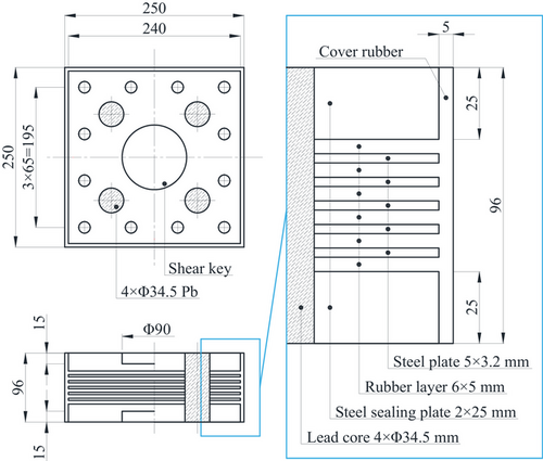
Six LHDR bearing specimens were designed and manufactured by Kawakin Co., Ltd. and tested in accordance with the JRA design specifications for highway bridges [21] and the manual of bearing in highway bridges [24]. Figure 1 illustrates the dimensions of the LHDR bearing, while Table 1 presents the parameters of the bearing. The specimen had a square cross-section of 240 mm × 240 mm and a shear modulus of 1.2 MPa. The LHDR bearing comprised six layers of high-damping rubber and five layers of steel plate, with thicknesses of 5 and 3.2 mm for each layer, respectively. Two steel sealing plates with a thickness of 25 mm were attached to the top and bottom surfaces. Four lead cores, each with a diameter of 34.5 mm, were embedded in the bearing to enhance energy dissipation capacity. The first and second shape factors of the specimen were 12 and 8, respectively.

Details are in the caption following the image — **FIGURE 1**
Open in figure viewer PowerPoint

Dimensions and thermocouple layout of LHDR bearing specimen (mm).

TABLE 1. Dimension and material properties of LHDR bearing specimens.

Parameter	Specification
$A$ , cross section (mm²)	240 × 240
${d}_l$ , diameter of lead core (mm)	34.5
${n}_l$ , number of lead core	4
${n}_r$ , number of HDR laminate	6
${t}_r$ , thickness of single HDR laminate (mm)	5
${n}_s$ , number of steel plate	5
${t}_s$ , thickness of single steel plate (mm)	3.2
$G$ , shear modulus (MPa)	1.2
${S}_1$ , first shape factor	12
${S}_2$ , second shape factor	8

2.2 Test Setup

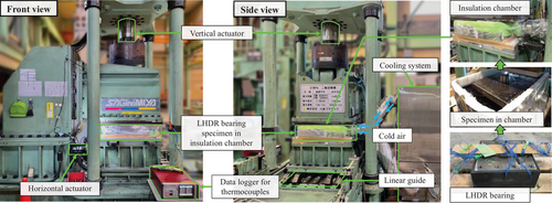
A two-axis testing machine was used to apply vertical compression and horizontal loading to the specimen, as shown in Figure 2. The specimen was fixed vertically and subjected to a compressive stress of 6 MPa. The displacement was applied by the horizontal actuator at the bottom, and the corresponding shear force was recorded by the load cell. Table 2 lists the loading capacity of the test setup. The maximum loading force, displacement, and speed of the vertical actuator in two directions were +1000/−2000 kN (tension/compression), ±150 mm, and 7 mm/s, respectively, while those of the horizontal actuator were ±400 kN, ±200 mm, and 630 mm/s, respectively.

TABLE 2. Loading capacity of test setup.

	Vertical direction	Horizontal direction
Maximum force	+1000/−2000 kN	±400 kN
Maximum displacement	±150 mm	±200 mm
Maximum speed	7 mm/s	630 mm/s

Three ambient temperature cases, −20°C, 0°C, and 23°C, were scheduled in the CL and HS test, according to the Manual of Bearings in Highway Bridges in Japan [24], to investigate the temperature-dependent property of the LHDR bearing. The specimen was covered by an insulation chamber. A cooling system was connected to the chamber by pipes to supply the cold air to maintain the specified constant ambient temperature within the chamber. The specimen was exposed to the ambient for 24 h before the test, according to the Manual of Bearings in Highway Bridges in Japan [24]. Note the factor of exposure duration at low temperatures was not considered in this research. The 24-h exposure time was set to ensure the internal temperature of the bearing matched the ambient temperature. The temperature inside the bearing was also confirmed by thermocouples set within the bearing. Once loading commenced, the internal temperature of the bearing increased due to the heating effect. This temperature variation was recorded using thermocouples to validate the accuracy of the subsequent temperature-dependent model.

2.3 Quasi-Static Cyclic Loading Test

The quasi-static CL test was conducted according to the JRA manual of bearing in highway bridges [24] for cyclic behavior analysis and further parameter identification of the restoring force model. The CL test arrangement of the LHDR bearing specimen is listed in Table 3. The scragging effect, which meant the initial stiffness of the bearing would be relatively large under the first cycle, was considered in this test, because it was a critical factor influencing the mechanical performance of the bearings, and its variation at low temperatures warranted attention [7]. The loading protocol is displacement control. Figure 3A shows the horizontal loading patterns without the cooling interval (CL-1st). The sinusoidal wave with a constant period of 8 s was applied to the specimen under −20°C, 0°C, and 23°C. The specimen experienced strain amplitudes of 50%, 100%, 150%, 200%, and 250% with five cycles at each level to simulate various earthquake intensities, according to the Japan Road Association: Specifications for highway bridges. Part V: Seismic design [21] to obtain the mechanical properties of the bearings, such as initial stiffness and yield displacement. This method has also been used to obtain the lower-bound properties of bearings [46]. Note that the sixth cycle with reduced strain amplitude was set after the fifth cycle to ensure the loading stopped smoothly. Figure 3B shows the horizontal loading patterns of cyclic loading considering the cooling interval (CL-2nd). The specimens underwent cyclic shear tests with a sinusoidal wave, where the period and amplitude were proportional, resulting in an average loading rate of 30 mm/s in each cycle. Intervals of approximately 1 h were set between loading cycles of different strain amplitudes to make sure the internal temperature of the bearing returned to the expected ambient temperature. Different from the first-time cyclic loading (CL-1st), setting the cooling interval in CL-2nd can improve the accuracy of the temperature variation within the bearing at different strain amplitudes and its impact on cyclic behavior. The introduction of intervals between loading cycles in CL-2nd was necessary to account for the significant temperature rise within the bearing at low temperatures, which affects mechanical properties. In CL-1st, continuous loading led to inaccurate results due to the neglect of the heating effect. Therefore, in CL-2nd, loading intervals were incorporated to more accurately capture the mechanical behavior of the bearings under low-temperature conditions. The temperature history of CL will be compared in Section 3.

TABLE 3. Test arrangement of LHDR bearing specimens.

Test	Loading pattern	23°C	0°C	−20°C	Scragging effect	Cooling interval
		Specimen
1	CL-1st	No. 1	No. 2	No. 3	Yes	No
1	HS-PD	No. 1	No. 2	No. 3	No	‒
2	HS-RT-1st	No. 4	No. 5	No. 6	Yes	‒
	CL-2nd	No. 4	No. 5	No. 6	No	Yes
	HS-RT-2nd	No. 4	No. 5	No. 6	No	‒

2.4 Hybrid Simulation Test

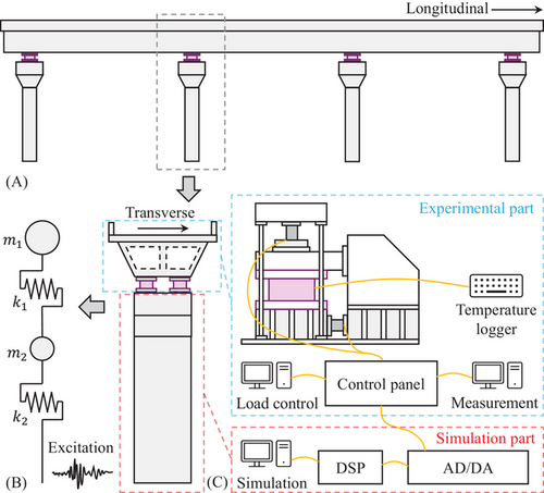
The hybrid simulation (HS) provides a cost-effective way to conduct irregular loading for structural performance testing. The HS test arrangement of the LHDR bearing specimen is also listed in Table 3. Figure 4 shows the framework of the HS test. A hypothetical three-span continuous girder bridge model with eight LHDR bearings (Figure 4A) was simplified into a two-degree-of-freedom (2-DOF) pier model (Figure 4B) with two bearings. It is assumed that the pier remains elastic in this model. The design parameters of the model are listed in Table 4. The HS system integrated experimental testing with numerical simulation, as illustrated in Figure 4C. The experimental loading and numerical simulation were conducted simultaneously based on the input ground motion. The experimental component comprised the scaled LHDR bearing and the simulated action of the bridge superstructure. The prototype bearing had a cross-section of 1440 mm × 1440 mm and a total rubber thickness of 180 mm. In the numerical component, the ground motion was applied to the numerical model. The equation of motion was integrated using the Newmark-beta scheme ( $\beta = 1/6$ ) within the digital signal processing (DSP) system to simulate the structural response. The load control computer recorded the signal of scaled displacement, which was subsequently converted into actuator loading instructions via the control panel. Another computer recorded the restoring force and displacement, and then transmitted the data to the DSP for seismic response correction of the bearing. This process was repeated until the time history analysis was completed. Meanwhile, the temperature within the bearing was monitored by thermocouples and recorded by a temperature logger.

TABLE 4. Parameters of the 2-DOF bridge model.

Parameter	Specification
${m}_1$ , mass of superstructure (t)	10,156
${m}_2$ , mass of pier (t)	3385
${k}_1$ , initial stiffness of bearing (kN/mm)	376
${k}_2$ , stiffness of pier (kN/mm)	400
$\xi$ , damping ratio	0.05
$T$ , natural period (s)	1.30

In this HS test, the User Interface on the PC was composed of Visual C#, and the DSP part program was coded by C [47, 48]. The motion equation of the structural model can be expressed as

\begin{equation} {\left[ M \right]\left\{ a \right\} + \left[ C \right]\left\{ v \right\} + \left[ K \right]\ \left\{ d \right\} = \left[ M \right]\ \left\{ {{a}_g} \right\}} \end{equation}

(1)

where

[ M ]

[ C ]

, and

[ K ]

were the matrices of the structural mass, damping, and stiffness;

\{ a \}

\{ v \}

, and

\{ d \}

were the acceleration, velocity, and displacement vectors of structure;

\{ {{a}_g} \}

was the acceleration of ground.

The motion equation of the system in increment form at time step

n + 1

can be expressed as

\begin{equation} {\left[ M \right]\left\{ {\Delta {a}_{n + 1}} \right\} + \left[ C \right]\left\{ {\Delta {v}_{n + 1}} \right\} + \left[ K \right]\left\{ {\Delta {d}_{n + 1}} \right\} = \left[ M \right]\left\{ {\Delta {a}_{g,n + 1}} \right\}} \end{equation}

(2)

where

\begin{equation} {\left\{ {\Delta {a}_{n + 1}} \right\} = \{ {a}_{n + 1}\ \} - \left\{ {{a}_n} \right\}} \end{equation}

(3)

\begin{equation} {\left\{ {\Delta {v}_{n + 1}} \right\} = \left\{ {{v}_{n + 1}} \right\}\ - \ \left\{ {{v}_n} \right\} = \left\{ {{a}_n} \right\}\Delta t + \frac{1}{2}\left\{ {\Delta {a}_{n + 1}} \right\}\Delta t} \end{equation}

(4)

\begin{equation} {\ \left\{ {{{\Delta}}{d}_{n + 1}} \right\} = \left\{ {{d}_{n + 1}} \right\} - \left\{ {{d}_n} \right\} = \left\{ {{v}_n} \right\}\Delta t + \frac{1}{2}\left\{ {\Delta {a}_n} \right\}\Delta {t}^2 + \beta \left\{ {\Delta {a}_{n + 1}} \right\}\Delta {t}^2} \end{equation}

(5)

Take Equations (3)–(5) into Equation (2), it can be written as

\begin{equation} {\left[ {\hat{M}\left] {\ \left\{ {{{\Delta}}{a}_{n + 1}} \right\} = \left[ M \right]\ \left\{ {{{\Delta}}{a}_{g,n + 1}} \right\} - \left[ {{A}_a} \right]\left\{ {{a}_n} \right\} - \left[ {{A}_v} \right]\ \left\{ {{v}_n} \right\} = } \right[\Delta \hat{F}} \right]} \end{equation}

(6)

where

\begin{equation} {\ \left[ {\hat{M}} \right] = \left[ M \right] + \frac{1}{2}\left[ C \right]\Delta t + \beta \left[ K \right]\Delta {t}^2} \end{equation}

(7)

\begin{equation} {\ \left[ {{A}_a} \right] = \left[ C \right]\Delta t + \frac{1}{2}\left[ K \right]\Delta {t}^2} \end{equation}

(8)

\begin{equation} {\ \left[ {{A}_v} \right] = \left[ K \right]\Delta t} \end{equation}

(9)

The predicted acceleration increment of the structure was

\begin{equation} {\ \left\{ {{{\Delta}}{a}_{p,n + 1}} \right\} = {{\left[ {\hat{M}} \right]}}^{ - 1}\ \left[ {\Delta \widehat {{F}_p}} \right]} \end{equation}

(10)

The predicted vertical and displacement increments

\{ {{{\Delta}}{v}_{p,n + 1}} \}

and

\{ {{{\Delta}}{d}_{p,n + 1}} \}

can be determined according to the Equations (4) and (5). However, the predicted values were still linear approximations and needed to be corrected for the following step analysis. Thus, the

[ K ]\{ {{{\Delta}}{d}_{n + 1}} \}

in Equation (1) was replaced by the actual

\{ {{{\Delta}}{f}_{n + 1}} \}

. The motion equation can be expressed as

\begin{align} &\left[ M \right]\left\{ {{{\Delta}}{a}_{n + 1}} \right\} + \left[ C \right]\left\{ {{{\Delta}}{v}_{n + 1}} \right\} + \left[ K \right]\left\{ {{{\Delta}}{d}_{n + 1}} \right\} \nonumber\\ &\quad + \left( {\left\{ {{{\Delta}}{f}_{n + 1}} \right\} - \left[ K \right]\left\{ {{{\Delta}}{d}_{n + 1}} \right\}} \right) = \left[ M \right]\ \left\{ {\Delta {a}_{g,n + 1}} \right\} \end{align}

(11)

The corrected force

\{ {{{\Delta}}{f}_c} \} = \{ {{{\Delta}}{f}_{n + 1}} \}\ - [ K ]\{ {{{\Delta}}{d}_{p,n + 1}} \}

, the corrected acceleration increment

\{ {{{\Delta}}{a}_{c,n + 1}} \} = {[ {\hat{M}} ]}^{ - 1}\ \{ {{{\Delta}}{f}_c} \}

. The actual acceleration can be calculated as

\begin{align} \left\{ {{{\Delta}}{a}_{n + 1}} \right\} &= {{\left[ {\hat{M}} \right]}}^{ - 1}\ \left[ {{{\Delta}}\widehat {{F}_p}} \right] - {{\left[ {\hat{M}} \right]}}^{ - 1}\ \left\{ {{{\Delta}}{f}_c} \right\} \nonumber\\ &= \left\{ {{{\Delta}}{a}_{p,n + 1}} \right\}\ - \left\{ {\Delta {a}_{c,n + 1}} \right\} \end{align}

(12)

The vectors of velocity and displacement

\{ {{{\Delta}}{v}_{n + 1}} \}

and

\{ {{{\Delta}}{d}_{n + 1}} \}

can be calculated as

\begin{equation} {\ \left\{ {{{\Delta}}{v}_{n + 1}} \right\} = \left\{ {{{\Delta}}{v}_{p,n + 1}} \right\} + \frac{1}{2}\left\{ {{{\Delta}}{v}_{c,n + 1}} \right\}\Delta t} \end{equation}

(13)

\begin{equation} {\ \left\{ {{{\Delta}}{d}_{n + 1}} \right\} = \left\{ {{{\Delta}}{d}_{p,n + 1}} \right\} + \beta \left\{ {{{\Delta}}{d}_{c,n + 1}} \right\}\Delta {t}^2} \end{equation}

(14)

After the correction, the computational accuracy of HS can be ensured.

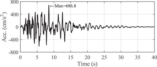
Figure 5 shows the input ground motion, which was Level-2, Type II, Ground-type II, Accelerogram 1 (II-II-1), specified by Specifications for highway bridges [21]. This ground motion was recorded from the 1995 Great Hanshin earthquake and belonged to the category of pulse-like near-fault earthquakes. It is also one of the near-fault ground motions specified for use in the seismic design of highway bridges in Japan. Two loading patterns with different rates were employed: pseudo-dynamic loading at a constant rate of 10 mm/s and real-time loading at the actual seismic rate, as shown in Figure 6. The pseudo-dynamic HS was conducted to prevent the bearing's maximum force from exceeding the testing device's capacity due to stiffness hardening. Although pseudo-dynamic loading was applied to seismic ground motions to obtain structural responses, it cannot accurately capture the response of the bearing under pulse-like near-fault earthquakes. For instance, in the case of the selected ground motion in Figure 5, the peak velocity acting on the bearing reached 324 mm/s, far exceeding the 10 mm/s rate used in pseudo-dynamic loading, as shown in Figure 6. Therefore, real-time HS was subsequently performed to capture the seismic response of the bearing under a real earthquake more accurately.

Two loading patterns with different rates were employed: pseudo-dynamic loading at a constant rate of 10 mm/s and real-time loading at an actual real-time rate, as shown in Figure 6. The pseudo-dynamic HS was performed to prevent the maximum force of the bearing from exceeding the loading capacity of the testing device caused by stiffness hardening. The real-time HS was conducted to investigate the actual seismic response of the bearing.

Kalpakidis and Constantinou [10] have proposed a similitude law and its validated theory for large and small bearings in complete and incomplete similarity. When the size of the bearing specimen is reduced, the loading velocity should be correspondingly increased in order to accurately capture the mechanical behavior of the bearing. Given the challenges of full-scale low-temperature testing and real-time loading, a reduced loading velocity was adopted as a balanced choice, considering equipment limitations, temperature control, internal temperature monitoring, and the dynamic behavior of the structural model and bearings. Table 5 presents the similitude law for the physical quantities of scaled specimens involved in the real-time HS in this research. Note that a reduced velocity would lead to an underestimation of the heat generated within the bearing.

TABLE 5. Similitude law for real-time hybrid simulation.

Physical quantity	Dimension	Scale factor	Note
Length/displacement	L	s
Mass	M	s³
Time	T	1	No time scale in real-time hybrid simulation
Stress	ML⁻¹T⁻²	s²→1	Consider rate dependence of stress
Strain	1	1
Force	MLT⁻²	s⁴→s²	Area times stress
Velocity	LT⁻¹	s
Acceleration	LT⁻²	s
Thermal diffusivity	L²T⁻¹	s²
Specific heat	1	1
Volumetric heat generation rate	T⁻¹	1
Temperature increment	T⁻¹	1

The real-time HS required synchronization of loading time between the experiment and the numerical simulation. Therefore, the time scale factor was set to 1. Moreover, due to the rate dependence of HDR material, stress in the bearing was assumed to scale consistently with the strain rate, with a scale factor of 1. Accordingly, force is obtained by multiplying the area by stress, and the scaling factor for force is

{s}^2

, and not driven form its dimension, which is related to the inertia force. In addition, since the heating effect can impact the mechanical performance of the bearings, scaling factors of thermodynamic-related physical quantities were also derived. The heat equation considering temperature conduction and heat generation within the bearings can be expressed as,

\begin{equation} {\ \frac{{\partial T\left( {x,t} \right)}}{{\partial t}} = \alpha \frac{{{\partial }^2T\left( {x,t} \right)}}{{\partial {x}^2}} + \frac{{{\dot{w}} ( t )}}{{c\rho }}} \end{equation}

(15)

where

\frac{{\partial T( {x,t} )}}{{\partial t}}

is the rate of change of temperature with respect to time;

\alpha

is the thermal diffusivity of the material,

\alpha = \frac{k}{{c\rho }}

;

\frac{{{\partial }^2T( {x,t} )}}{{\partial {x}^2}}

represents the one-dimensional heat conduction. For the lead core, it can be assumed that the temperature inside the lead core is uniform, so this term is zero.

{\dot{w}} ( t )

is the volumetric heat generation rate (heat generation per unit volume per unit time), which can be expressed as

w\ ( t ) = \int _0^t \sigma ( \tau ){\dot{\varepsilon}} ( \tau )d\tau

;

c

and

\rho

are specific heat and density of materials, respectively. Table 6 lists the thermal properties of materials in this model. Based on dimensional analysis (the dimensions on both sides of Equation 15 should be the same), it can be determined that the scaling factor for the internal temperature increment (unit time) of the bearing in real-time hybrid experiments is 1. Note that in this study, the internal temperatures were compared at 23°C, 0°C, and −20°C; however, there was a concern that they may not have been fully reproduced, and full-scale testing will be necessary in the future.

TABLE 6. Thermal properties of materials.

Material	Lead	Steel	HDR
$k$ , thermal conductivity [W/(m·K)]	35.30	38.76	0.31
$c$ , specific heat [J/(kg·K)]	129	432	1732
$\rho$ , density (kg/m³)	11,360	7740	1146
$\alpha$ , thermal diffusivity (m²/s)	2.41×10⁻⁵	1.16×10⁻⁵	1.56×10⁻⁷

3 Experimental Results

3.1 Cyclic Loading Test

3.1.1 Hysteretic Behavior

The hysteresis curves of specimens under 1st and 2nd CLs at −20°C, 0°C, and 23°C were compared in Figure 7. In general, the temperature showed a significant effect on the hysteretic behavior of the LHDR bearing. As the ambient temperature decreased, the maximum stress, the area of the covered loops, and the initial stiffness of the bearing increased.

Moreover, differences can be found between the two CLs due to the scragging effect. In CL-1st, since the specimen was in the first-time loading (or initial loading), the larger stress and stiffness can be observed in the first cycle loading at each strain amplitude. For instance, in CL-1st, the stress and stiffness of the specimen in the first cycle at 100% were larger than those in the second cycle. As the loading reached the amplitude of 150%, the path of the loop in the first cycle could not follow, but was below the loop in the first cycle at 100%. Only when the loading strain exceeded 100%, the stress and stiffness of the specimen increased rapidly. This behavior is attributed to the scragging effect, which refers to the initial softening of the material, where the stiffness and stress decrease after the first loading cycle due to internal molecular rearrangements in the rubber. However, in CL-2nd, the loop in the first cycle at a certain amplitude just followed the loop in the first cycle at the previous amplitude due to the elimination of the scragging effect. This effect is typically eliminated after the initial loading cycles, as the internal structure of the rubber stabilizes and further molecular rearrangements become negligible. As a result, the mechanical response becomes more repeatable in subsequent cycles.

It should be noted that in CL-2nd loading at −20°C, the expected strain of the first cycle at 200% and 250% strain amplitudes was not achieved due to the maximum horizontal restoring force of the specimen exceeding the test range of the loading machine (400 kN in horizontal loading in Table 2).

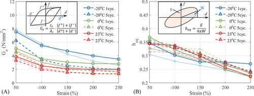
The equivalent shear modulus and damping ratio of the specimen under CLs at −20°C, 0°C, and 23°C are shown in Figure 8. The bold lines represented the CL-2nd loading, while the thin lines with the light color represented the CL-1st loading. As the ambient temperature decreased, the equivalent shear modulus showed a significant increase, because the HDR became stiffer and less flexible at low temperature. Especially at −20°C, the shear modulus of the bearing in the first cycle was twice that at 23°C, which would affect the hysteretic behavior and the effectiveness of the isolation system. For the equivalent damping ratio, the temperature had no notable effect on it. As the temperature decreased, the restoring force of the bearing increased, and it increased proportionally with the energy dissipated per cycle. Moreover, the equivalent shear modulus and damping ratio decreased with the increase of loading cycles at the same strain level and the increase of the strain amplitude. That is because the material underwent degradation, due to repeated loading, which led to a decrease in stiffness and energy dissipation capacity.

3.1.2 Temperature History

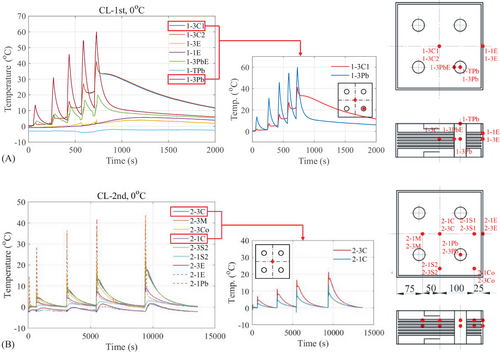
The temperature history of LHDR bearing under 1st and 2nd cyclic loadings (CL-1st and CL-2nd) at 0°C was shown as an example in Figure 9. The cooling intervals were applied in CL-2nd but not in CL-1st. Due to the limited heat transfer within a short period, the temperature rise of the rubber and lead core inside the bearing in CL-1st was significantly higher than that in CL-2nd. The temperature variation within the lead core was more rapid than that of rubber because the thermal conductivity of lead was much higher than that of rubber. Moreover, a significant temperature difference was observed between the first and third rubber layers because heat accumulated in the middle layer and transferred outward, while the heat in the outer layer dissipated rapidly through the steel plate. The notable temperature differences between rubber layers may lead to localized damage. For example, the middle rubber layer, having a higher temperature, exhibits lower stiffness and larger strain, making it more likely to reach the critical shear strain for failure first. Given the temperature sensitivity of rubber, it is essential to evaluate the effect of the temperature differences on the mechanical properties of the bearing, highlighting the need for further investigation. Additionally, the temperature difference at different positions in the same layer can be observed. The temperature difference in the third layer was smaller than that in the first layer.

3.2 Hybrid Simulation Test Results and Discussion

3.2.1 Hysteretic Behavior

The hysteresis curves of the specimen under real-time and pseudo-dynamic hybrid simulations (HS-RT-1st, HS-RT-2nd, and HS-PD) at −20°C, 0°C, and 23°C were compared in Figure 10. As the ambient temperature decreased, the initial stiffness of the specimen increased, increasing maximum force (absolute maximum shear force recorded in the hysteresis curve) and area of loops. A significant increase can be found in real-time loading, especially for the first-time real-time loading (HS-RT-1st).

As for the effect of loading rate, the specimen presented a larger force in real-time loading (HS-RT-2nd) compared with that in pseudo-dynamic loading (HS-PD), with the elimination of the scragging effect. The maximum force in HS-PD loading was slightly lower than that in HS-RT-2nd. Moreover, the curve became smoother at the position where the loading direction changed. Due to the rate dependence of the rubber bearing, low-rate seismic loading may cause the underestimation of the hysteretic behavior of the bearing.

The scragging effect was another point worth discussing. The specimen showed a larger force in the first-time real-time loading (HS-RT-1st) compared with the second-time loading (HS-RT-2nd). The reason was that the friction along a certain direction in the rubber was weakened after the initial cycle, leading to a long-term degradation in the stiffness of the bearing. When applying such a type of isolation bearing, especially in low-temperature regions, sufficient attention should be given to the scragging effect.

3.2.2 Temperature History

The temperature history of the specimen under real-time and pseudo-dynamic hybrid simulations (HS-RT-2nd and HS-PD) at −20°C,0°C, and 23°C was illustrated in Figure 11. As the ambient temperature decreased, the temperature increment of the specimen increased. Owing to the increase in the stiffness of the bearing at low temperatures, the area of the hysteresis loop (or dissipated energy) increased, resulting in a larger temperature increment. Moreover, the temperature increment rose in the real-time HS due to the time-dependent heat generation and conduction.

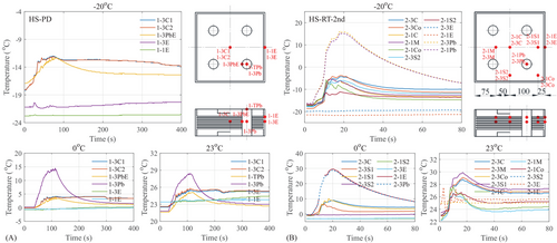
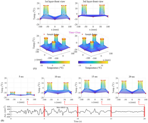
Figure 12 shows a three-dimensional temperature distribution of LHDR bearing under real-time hybrid simulation (HS-RT-2nd) at −20°C. In Figure 12A, the temperature difference between the 1st and 3rd rubber layers can be observed during the HS. Although the temperature difference in HS was not as large as that in CL (e.g., at the ambient temperature of 0°C, the temperature difference is 10°C in CL but 5°C in HS), it may still lead to local damage due to the non-uniform strain distribution across the bearing layers. A thermo-mechanical coupling model may need to evaluate this difference. It was interesting to note that the initial stiffness of the bearing increased with decreasing ambient temperature, while the stiffness decreased with the rise of internal temperature during loading. The decreased stiffness owing to the heating effect seemed to be beneficial to the effectiveness of the isolation system. However, for pulse-like near-fault ground motions (e.g., the selected input ground motion), the internal temperature of the bearing did not show a significant rise when the seismic acceleration reached the peak. In fact, even when the ground motion ends, the internal temperature may still not reach room temperature. The low-temperature effect still dominated, resulting in a relatively high stiffness of the bearing. For instance, Figure 12B depicts the temperature distribution of 1st rubber layer of the specimen under real-time loading at −20°C according to the recorded temperature data. The maximum acceleration of ground motion was at the 8-s. The temperature of the rubber was near −15°C and −5°C at the 5 and 10-s, while it was still below 0°C after 20 s, which is far below the room temperature. Additionally, the scale effect may also affect the heat conduction within the bearing. When the loading time is scaled, the heat generation in the bearing is affected by the scaling factor, making it inaccurate to predict the full-scale heat generation using a scaled model [10]. However, in the condition of real-time HS in this study, the time scaling factor is 1. Considering that stress is proportional to strain rate, the stress scaling factor is also 1. As derived from Table 5, the temperature increment scaling factor is 1, indicating that temperature variation is independent of the bearing size. In general, the low temperature had a significant impact on the hysteretic behavior of the bearing, even though the heating effect was considered.

3.2.3 Energy Dissipation

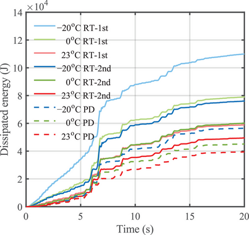
The energy dissipation of the specimen under real-time and pseudo-dynamic hybrid simulations (HS-RT-1st, HS-RT-2nd, and HS-PD) at −20°C, 0°C, and 23°C was shown in Figure 13. Consistent with the analysis of the hysteretic behavior, the energy dissipation of the bearing increased as the temperature decreased. However, some research on numerical simulation [25] found that the energy dissipation of the bearing decreased at lower temperatures. Note that the behavior of the pier in the bridge model was assumed to be linear elastic in this HS, while in the mentioned research, the pier exhibited elastoplastic behavior. The yielding of the pier would possibly reduce the displacement demand of the isolated bearings.

3.2.4 Seismic Response of Structure

The seismic responses of the hypothetical bridge model, including the superstructure and pier, were analyzed to investigate the effects of low temperature, loading rate, and scragging on the structure.

The absolute displacement and acceleration of the superstructure under real-time and pseudo-dynamic hybrid simulations (HS-RT-1st, HS-RT-2nd, and HS-PD) were compared in Figures 14 and 15. The response of the superstructure is minimally affected by temperature, loading rate, and scragging. The absolute displacement of the superstructure increased as the ambient temperature decreased, which needed to be considered to prevent collisions between the abutment and the superstructure. Moreover, the absolute acceleration of the superstructure was slightly amplified at low temperatures.

The displacement of the pier under real-time and pseudo-dynamic hybrid simulations (HS-RT-1st, HS-RT-2nd, and HS-PD) was compared in Figure 16. The temperature effect showed a significant impact on the response of the pier. The maximum displacements of the pier top increased by 71.2%, 90.0%, and 120.7% at −20°C compared with those in 23°C under RT-1st, RT-2nd, and PD loadings, respectively. Note that in the hypothetical model, the pier was assumed to be elastic. It can be inferred that the difference in the pier top displacement would be larger when the yielding happened on the pier. This was quite dangerous for the bridge, potentially even posing pier failure. The scragging effect led to a greater response of the structure, including the maximum displacement, acceleration, and force of the pier.

In general, low-temperature environments lead to an increase in the stiffness of LHDR bearings, resulting in higher restoring forces. Consequently, the effectiveness of the isolation system is weakened, as reflected in the increased displacement at the bridge pier top. Therefore, when designing seismic isolation structures in cold regions, it is essential to consider the impact of temperature on seismic performance. This includes establishing the relationship between temperature and the equivalent shear stiffness and damping ratio of the bearings, as well as accounting for the variations in mechanical properties within the temperature range of cold regions.

4 Proposed Model and Model Validation

4.1 Numerical Model

A rate-dependent multi-layer thermo-mechanical Bouc–Wen (MTBW) model was developed by Shen et al. [45] to simulate the hysteretic behavior of LHDR bearings. This model illustrates the internal heat transfer mechanism as well as the rate dependence. However, the scragging effect of the bearing cannot be expressed in this model. The rate-dependent MTBW model is extended in this section to further consider the scragging effect. The proposed model is illustrated in Figure 17.

The restoring force and displacement relationship of the MTBW model can be expressed as

\begin{align} {f}_r ( t ) &= {\alpha }_1\ {e}^{{m}_r \times \frac{{{T}_r( t ) - 23}}{{100}}}{K}_r{d}_r( t ) \nonumber\\ &\quad + \left[ {1 + b{\varepsilon }_r\left( {{{\left. t \right)}}^2} \right.} \right]\left( {1 - {\alpha }_1} \right){e}^{{n}_r \times \frac{{{T}_r( t ) - 23}}{{100}}}{K}_r{Z}_r( t ) \end{align}

(16)

where

\begin{equation} {{{{\dot{Z}} }}_r( t ) = {{{\dot{d}} }}_r\ ( t ) - \beta | {{{{\dot{d}} }}_r( {\mathrm{t}} ){Z}_r( {\mathrm{t}} )} |{Z}_r( t ) - \gamma {{{\dot{d}} }}_r( t )Z_r^2( t )} \end{equation}

(17)

\begin{equation} {\beta = \frac{1}{{\left( {1 + s} \right)d_y^2}}\ } \end{equation}

(18)

\begin{equation} \gamma =s\cdot \beta \end{equation}

(19)

where

{\alpha }_1

is the post-yielding stiffness ratio;

{m}_r

and

{n}_r

are parameters describing temperature dependence;

{T}_r( t )

is the temperature at the center of single HDR laminate;

{K}_r

is the initial stiffness of each HDR laminate;

{d}_r( t )

and

{\varepsilon }_r( t )

are the input horizontal displacement and corresponding strain of each HDR laminate;

{t}_r

is the thickness of each HDR laminate;

{Z}_r( t )

is the hysteretic component of restoring force of each HDR laminate;

b

\beta

\gamma

, and

s

are dimensionless parameters of hysteresis curve;

{d}_y

is the yield displacement.

The rate dependence is represented by a dashpot and a spring in series (Maxwell model), with the parameters of the dashpot constant (

{c}_v

) and the spring constant (

{K}_v

). The restoring force related to the rate dependence (

{f}_v

) can be expressed as

\begin{equation} {\ {f}_v = {c}_v\ {{{\dot{d}} }}_d = {K}_v\ {d}_s} \end{equation}

(20)

where

{d}_d

is the displacement of the dashpot;

{d}_s

is the displacement of the spring. The sum of

{d}_d

and

{d}_s

should be the total displacement of the LHDR bearing (

d

), written as

\begin{equation} {d = {d}_d + {d}_s} \end{equation}

(21)

Tan et al. [9] proposed a random polymer model to illustrate the stress-softening behavior of HDR bearings. The Mullins effect was explained in this model by a coefficient to the nonlinear term of the restoring force model. This mechanism is added to the existing rate-dependent MTBW model to simulate the scragging effect. The scragging effect is assumed to be caused by the friction generated in the movement of polymer chains in the rubber within a certain range. These frictional forces are weakened as the polymer chains move back and forth against each other. The restoring force related to the scragging effect (

{f}_i

) can be expressed as

\begin{equation} {{f}_i\ ( t ) = \left[ {1 + g\left( {\varepsilon ,t} \right)} \right]\ \left( {1 - {\alpha }_1} \right){e}^{{n}_r \times \frac{{{T}_r( t ) - 23}}{{100}}}{K}_r{Z}_r( t )} \end{equation}

(22)

where

g( {\varepsilon,t} )

is the coefficient of fraction force related to the scragging effect, which is controlled by two parameters

p

and

q

. The detailed mechanism can be found in the reference [9].

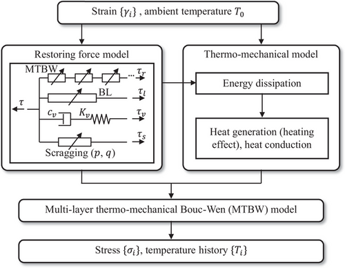
In addition, the hysteretic behavior of the lead core is indicated by the bilinear (BL) model mode, with the parameters of initial stiffness ( ${K}_l$ ) and characteristic strength ( ${Q}_l = 11.21$ kN).

The total restoring force of the rubber bearing (

f

) can be obtained by adding the HDR laminate (

{f}_r

), rate dependence (

{f}_v

), lead core (

{f}_l

), and scragging effect (

{f}_s

) parts, as

\begin{equation} {f = {f}_r + {f}_v + {f}_l + {f}_s} \end{equation}

(23)

Regarding the heating effect in the HDR and lead core, we formulated the heat conduction mechanism based on the heat conduction equation, Equation (15), and coupled it into the restoring force model. It is important to note that heat transfer in the LHDR bearing was considered only in the vertical one-dimensional direction, while the heat conduction mechanism in the lead core followed the approach outlined in Reference [40]. The specific modeling assumptions can be found in Reference [45].

To obtain the parameters of the proposed model, an optimization algorithm, named the KH method [49, 50], was adopted. This method inputs the initial parameters and CL data, adjusting parameters to maximize the correlation coefficient ( ${R}^2$ ) within the set error to obtain the identified parameters. The identified parameters are then used to predict the performance of the bearing under dynamic loading, verifying the accuracy of the model. Note that only one set of parameters is needed to predict the performance of a bearing under three ambient temperatures. The identified parameters in this research will be shown in the next section.

4.2 Cyclic Loading Validation

4.2.1 Hysteretic Behavior

Figure 18 compares the hysteresis curves under CL between the results of the experiment and the numerical model. Specifically, Figure 18A shows the validation of the first cyclic loading (CL-1st), where the loading was with the scragging effect but without the cooling interval between strain amplitudes. When considering the scragging effect, the hysteresis curve exhibited a relatively larger stiffness and stress in the first cycle loading of a certain strain amplitude (e.g., 100%) and showed a decreasing trend in the second to fifth cycles. As the loading stepped to the next strain amplitude (e.g., 150%), the curve of the first cycle showed a lower stiffness compared with that in the previous strain level (e.g., 100%). However, the stress increased abruptly when the strain exceeded the previous strain level (e.g., 100%). The so-called scragging effect was well-captured with the proposed model. In addition, Figure 18B compares the second cyclic loading (CL-2nd), where the scragging effect was excluded, but the cooling interval was set. This result captured the characteristics of that hysteresis curve following the path of the previous strain level. In general, the proposed model can accurately reflect the mechanical behavior of the bearings under different ambient temperatures. Note that in Figure 18A, under CL-1st at −20°C, the hysteresis curves obtained from numerical analysis underestimated the peak stress in the first cycle at 100%–200% strain amplitudes. This discrepancy can be attributed to two factors: (1) In the experiment, as the strain amplitude increases, the peak stress of the bearing is expected to increase accordingly. However, the black curve showed that the peak stress remained almost unchanged, starting from 150% strain. This is likely due to the absence of cooling intervals in the loading protocol of the first test, which led to internal heat accumulation and, consequently, a reduction in bearing stiffness; (2) The parameter optimization method used in the present model is based on the coefficient of determination ( $R^2$ ), which prioritizes the overall fitting accuracy of the data. As a result, a discrepancy occurs in the fitting of peak values.

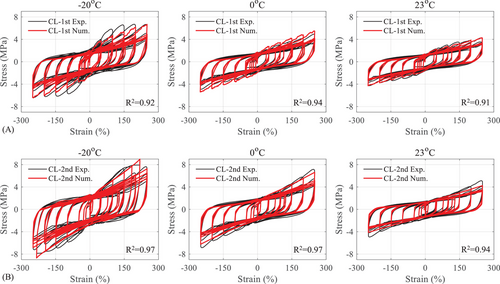
Table 7 lists the identified parameters of the model from CL-1st and CL-2nd. Regarding parameter sensitivity analysis, note that parameter $b$ has a significant impact on the shape of the curve. This parameter is the shape parameter of the nonlinear part of the restoring force model, used to represent the stiffness hardening of LHDR bearings. An appropriate initial value needs to be selected. Additionally, the parameters ${c}_v$ and ${K}_v$ in the rate-dependent part are negatively correlated with each other and require suitable initial values to be set.

TABLE 7. Identified parameters of the model from CL-1st and CL-2nd.

{\alpha }_1

${K}_r$

(kN/mm)

s

${d}_y$

(mm)

b

{m}_r

{n}_r

p

q

{c}_v

${K}_v$

(kN/mm)

${K}_l$

(kN/mm)

CL-1st

0.33

23.69

−0.77

1.26

0.34

−0.80

−2.01

0.05

0.30

0.20

2.00

22.07

CL-2nd

0.30

26.55

−0.80

1.24

0.35

−1.88

−3.21

‒

0.21

1.89

22.07

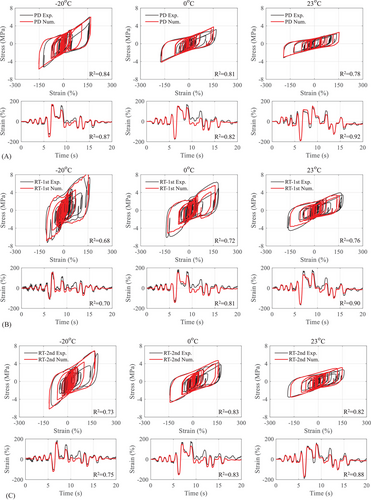
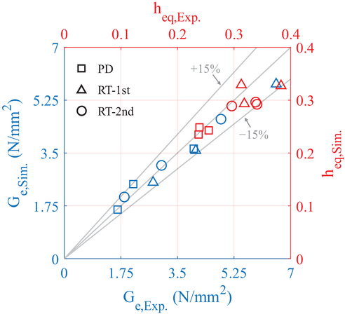
Figure 19 compares the equivalent shear modulus and damping ratio of the first, second, and fifth cycles of five strain levels in two cyclic loadings (CL-1st and CL-2nd). The error between the simulation and the experimental values is within 15%, indicating the model can predict the characteristics of the hysteretic behavior with decent accuracy.

4.2.2 Temperature History

Figure 20 compares the temperature history of the LHDR bearing under 1st and 2nd cyclic loadings (CL-1st and CL-2nd). The temperature prediction of specimens at 0°C was presented. The proposed model could well capture the temperature time history of the HDR laminates and lead core. Note that the temperature distribution of the same layer of rubber may be different, but this was ignored in the model for simplicity. In addition, in CL-1st, the cooling intervals were not sufficient. Thus, the initial temperature within the bearing was higher than the ambient temperature in large strain amplitudes. However, in CL-2nd, the initial temperature was the ambient temperature, resulting in a larger stiffness and stress in the first cycle loading for each strain amplitude compared with those in CL-1st.

4.3 Hybrid Simulation Validation

4.3.1 Hysteresis Behavior

Figure 21 depicts the hysteresis curve and strain time history of the LHDR bearing under the pseudo-dynamic and real-time HSs. With the consideration of the scragging effect and rate dependence, the proposed model could predict the hysteretic characteristic of the LHDR bearing, including the maximum stress and the strain time history, exhibiting high R² values. Figure 22 shows the validation of the equivalent shear modulus and damping ratio of the maximum loop. All equivalent shear stiffness and damping ratios fall within the 15% error range. It further demonstrated that the MTBW model can accurately predict the critical aspect of the LHDR bearing response under earthquakes, namely, the behavior of the maximum loop. Table 8 lists the parameters of the model used in HSs, which were identified from the CLs.

TABLE 8. Parameters of the model used in hybrid simulations.

	${\alpha }_1$	${K}_r$ (kN/mm)	$s$	${d}_y$ (mm)	$b$	${m}_r$	${n}_r$	$p$	$q$	${c}_v$	${K}_v$ (kN/mm)	${K}_l$ (kN/mm)
HS-PD	0.33	23.59	−0.77	1.26	0.34	−1.87	−3.22	‒	‒	0.20	2.00	22.07
HS-RT-1st	0.30	26.55	−0.80	1.24	0.35	−1.88	−3.21	0.05	0.30	0.20	2.00	22.07
HS-RT-2nd	0.30	26.55	−0.80	1.24	0.35	−1.88	−3.21	‒	‒	0.20	2.00	22.07

4.3.2 Temperature History

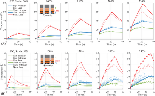
Figure 23 compares the temperature history of the LHDR bearing at 0°C under HSs. The proposed model could predict the temperature history of HDR laminates and lead core with decent accuracy. It found that the temperature increment was higher in real-time loading, especially in first-time loading, compared with the pseudo-dynamic loading. The loading rate and scragging effect were two main factors affecting the temperature history of the LHDR bearing.

4.3.3 Response of Structure

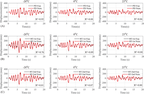
Figure 24 validates the displacement of the pier top under HS. The numerical results of the model showed good agreement with the test ones, exhibiting high R² values. The increased displacement of the pier top due to the decreased temperature was well captured. Moreover, the scragging effect and rate dependence were also simulated in the response of the pier top.

5 Conclusion

In this paper, the experimental investigation of the seismic performance of LHDR bearings at low temperatures was conducted. The CL tests with and without the cooling interval were compared to evaluate the hysteretic behavior and temperature effect of the bearings at −20°C, 0°C, and 23°C. Real-time and pseudo-dynamic HSs were then conducted to investigate the seismic performance of LHDR bearings and the response of the isolated bridge under realistic ground motion. A modified thermo-coupled restoring force model was proposed to simulate hysteretic behavior, considering the scragging effect and loading rate. The main conclusions can be drawn as follows:

The temperature effect on the behavior of LHDR bearings was significant, especially at low temperatures. The initial stiffness and maximum stress of the bearings showed a substantial increase as the temperature decreased. During CL, the equivalent shear modulus of the bearing was at −20°C twice that at 23°C. The seismic response of the isolated bridge was significantly affected by the temperature effect. The effectiveness of the isolation system weakened at low temperatures, as evidenced by the reduced lateral flexibility of the bearings. The displacement of the pier top increased significantly at −20°C. It is recommended to consider the effect of low temperatures during seismic design and to select appropriate isolation devices in low-temperature earthquake-prone regions.
The loading rate impacted the hysteretic behavior of LHDR bearings, including the maximum stress and temperature increment. The high-damping rubber exhibited rate-dependent characteristics, which affected the behavior of the bearing. A higher loading rate led to a larger response from the isolated bridge.
The scragging effect needed to be considered in the seismic performance evaluation of isolated bearings. The bearing exhibited larger stress during the first-time loading in both CL and HS. The structural response was also amplified under the initial loading.
The hysteretic behavior and temperature history were well predicted by the proposed modified thermo-coupled model, including the factors of scragging effect and rate dependence. In CLs, the scragging effect was simulated by the model, with the relatively large stiffness in the new strain history. The identified parameters were used in the HSs. In addition, the hysteretic behavior in the HS was performed well by this model, with the scragging effect in the comparison of the first and second real-time HSs, and the rate dependence in the comparison of the pseudo-dynamic and the first real-time HSs.

This study also has certain limitations and identifies directions for further research as follows:

In this research, 1/6-scaled LHDR bearings were used in the experimental investigation to consider the loading capacity of the test machine. The low-rate loading does not strictly follow the established similitude law proposed in reference [10], which may lead to an underestimation of the heat generation in the bearing. In addition, the scaling effect will affect the volume-to-surface ratio of the bearing. Thus, the temperature history of large-sized bearings cannot be directly predicted according to the scaled specimens.
Moreover, prolonged exposure to low temperatures may alter the seismic performance of LHDR bearings, which is also an important and worthwhile topic for further research. Although the oxidation rate of the bearing may slow down at low temperatures, polymer stiffening, and lead core fatigue are likely to intensify under low-temperature conditions.
This study selected a representative near-fault earthquake (the 1995 Hanshin Earthquake) based on the Specifications for highway bridges. Part V: Seismic design. However, to further understand the low-temperature dynamic behavior of the bearings, additional earthquake records should be tested. Furthermore, the long-duration earthquake also needs to be considered through an increased number of loading cycles or by applying long-period seismic inputs. As the heating effect in the bearings significantly affects their mechanical performance, long-period earthquakes can cause sustained energy dissipation in the bearing, leading to a continuous rise in internal temperature, which in turn affects its mechanical performance.

Acknowledgments

The authors have nothing to report.

Open Research

Data Availability Statement

The data that support the findings of this study are available from the corresponding author upon reasonable request.

References

1J. L. Gimenez and T. Himeno, “Seismic Isolation of Bridges Using Rubber Bearings with High Energy Dissipation Capacity,” in 20th ASEP Int. Convention: “Structural Engineering: Getting Smarter to New and Future Challenges” (2021).
Google Scholar
2K. N. G. Fuller, J. Gough, and A. G. Thomas, “The Effect of Low-Temperature Crystallization on the Mechanical Behavior of Rubber,” Journal of Polymer Science Part B: Polymer Physics 42, no. 11 (2004): 2181–2190.
10.1002/polb.20091
CAS Web of Science® Google Scholar
3W. Roeder Charles, F. Stanton John, and T. Feller, “Low-Temperature Performance of Elastomeric Bearings,” Journal of Cold Regions Engineering 4, no. 3 (1990): 113–132.
10.1061/(ASCE)0887-381X(1990)4:3(113)
Google Scholar
4T. Saito, S. Irie, Y. Nakamura, K. Takenouchi, Y. Miyamori, and T. Yamazaki, “Mechanical Characteristics of High Damping Rubber Bearings by Dynamic Loading Tests Under the Low Temperature Environment,” Journal of Japan Society of Civil Engineers, Ser A1 (Structural Engineering & Earthquake Engineering (SE/EE)) 37 (2018): 765–776.
10.2208/jscejseee.74.I_765
Google Scholar
5S. Nagarajaiah, M. Reinhorn Andrei, and C. Constantinou Michalakis, “Nonlinear Dynamic Analysis of 3-D-Base-Isolated Structures,” Journal of Structural Engineering 117, no. 7 (1991): 2035–2054.
10.1061/(ASCE)0733-9445(1991)117:7(2035)
Web of Science® Google Scholar
6D. A. Nguyen, J. Dang, Y. Okui, A. Amin, S. Okada, and T. Imai, “An Improved Rheology Model for the Description of the Rate-Dependent Cyclic Behavior of High Damping Rubber Bearings,” Soil Dynamics and Earthquake Engineering 77 (2015): 416–431.
10.1016/j.soildyn.2015.06.001
Web of Science® Google Scholar
7J. A. Gallardo, J. C. de la Llera, J. I. Restrepo, and M. Chen, “A Numerical Model for Non-Linear Shear Behavior of High Damping Rubber Bearings,” Engineering Structures 289 (2023): 116234.
10.1016/j.engstruct.2023.116234
Web of Science® Google Scholar
8A. Dall'Asta and L. Ragni, “Experimental Tests and Analytical Model of High Damping Rubber Dissipating Devices,” Engineering Structures 28, no. 13 (2006): 1874–1884.
10.1016/j.engstruct.2006.03.025
Web of Science® Google Scholar
9Y. Tan, Y. Liu, J. Dang, A. Igarashi, T. Himeno, and Y. Hamada, “Stress-Softening Behavior of High-Damping Rubber Bearings at Low Temperatures,” Journal of Structural Engineering 150, no. 6 (2024): 04024050.
10.1061/JSENDH.STENG-13253
Web of Science® Google Scholar
10I. V. Kalpakidis and M. C. Constantinou, “Principles of Scaling and Similarity for Testing of Lead–Rubber Bearings,” Earthquake Engineering and Structural Dynamics 39, no. 13 (2010): 1551–1568.
10.1002/eqe.1041
Web of Science® Google Scholar
11N. Murota and T. Mori, “An Experimental Study on Scale Effect in Dynamic Shear Properties of High-Damping Rubber Bearings,” Frontiers in Built Environment 6 (2020): 37.
10.3389/fbuil.2020.00037
Web of Science® Google Scholar
12E. Takaoka, Y. Takenaka, A. Kondo, M. Hikita, and H. Kitamura, “Heat-Mechanics Interaction Behavior of Laminated Rubber Bearings Under Large and Cyclic Lateral Deformation,” in 14th Conference on Earthquake Engineering (Beijing, China, 2008).
Google Scholar
13A. Yakut and J. A. Yura, “Parameters Influencing Performance of Elastomeric Bearings at Low Temperatures,” Journal of Structural Engineering 128, no. 8 (2002): 986–994.
10.1061/(ASCE)0733-9445(2002)128:8(986)
Google Scholar
14D. Cardone, G. Gesualdi, and D. Nigro, “Effects of Air Temperature on the Cyclic Behavior of Elastomeric Seismic Isolators,” Bulletin of Earthquake Engineering 9, no. 4 (2011): 1227–1255.
10.1007/s10518-011-9244-8
Web of Science® Google Scholar
15R. Zhang and A. Li, “Experimental Study on Temperature Dependence of Mechanical Properties of Scaled High-Performance Rubber Bearings,” Composites, Part B 190 (2020): 107932.
10.1016/j.compositesb.2020.107932
CAS Web of Science® Google Scholar
16C. Yasar, V. Karuk, E. Cavdar, and G. Ozdemir, “Modifications in both Lead and Rubber Properties of LRBs at Low Temperatures Considering the Size Effect,” Engineering Structures 307 (2024): 117902.
10.1016/j.engstruct.2024.117902
Web of Science® Google Scholar
17C. Yaşar, V. Karuk, E. Cavdar, and G. Ozdemir, “Variation in Mechanical Properties of a Lead–Rubber Bearing Exposed to Low Temperature,” Journal of Cold Regions Engineering 37, no. 3 (2023): 04023012.
10.1061/JCRGEI.CRENG-698
Web of Science® Google Scholar
18C. Yasar, V. Karuk, O. Kaplan, E. Cavdar, and G. Ozdemir, “Amplification in Mechanical Properties of a Lead Rubber Bearing for Various Exposure Times to Low Temperature,” Buildings 13, no. 2 (2023): 478.
10.3390/buildings13020478
Web of Science® Google Scholar
19V. Karuk, C. Yaşar, E. Çavdar, and G. Özdemir, “Combined Effect of Low Temperature and Exposure Time on Seismic Performance of an LRB-Isolated Bridge,” Journal of Bridge Engineering 29, no. 12 (2024): 04024092.
10.1061/JBENF2.BEENG-6608
Web of Science® Google Scholar
20E. Çavdar, G. Özdemir, and V. Karuk, “Modification in Response of a Bridge Seismically Isolated with Lead Rubber Bearings Exposed to Low Temperature,” Teknik Dergi 33, no. 5 (2022): 12553–12576.
10.18400/tekderg.880787
Web of Science® Google Scholar
21 JRA. Japan Road Association: Specifications for Highway Bridges. Part V: Seismic Design (Maruzen, 2019).
Google Scholar
22 AASHTO. American Association of State Highway and Transportation Officials: Guide Specifications for Seismic Isolation Design (AASHTO, 2014).
Google Scholar
23 CSA. CAN/CSA-S6-14: Canadian Highway Bridge Design Code (Canadian Standard Association, 2014).
Google Scholar
24 JRA. Japan Road Association: Manual of Bearing in Highway Bridges (Maruzen, 2018).
Google Scholar
25A. Billah and B. Todorov, “Effects of Subfreezing Temperature on the Seismic Response of Lead Rubber Bearing Isolated Bridge,” Soil Dynamics and Earthquake Engineering 126 (2019): 105814.
10.1016/j.soildyn.2019.105814
Web of Science® Google Scholar
26P. Deng, Z. Gan, T. Hayashikawa, and T Matsumoto, “Seismic Response of Highway Viaducts Equipped with Lead–Rubber Bearings Under Low Temperature,” Engineering Structures 209 (2020): 110008.
10.1016/j.engstruct.2019.110008
Web of Science® Google Scholar
27H. Wang, W.-Z. Zheng, J. Li, and Y.-Q. Gao, “Effects of Temperature and Lead Core Heating on Response of Seismically Isolated Bridges Under Near-Fault Excitations,” Advances in Structural Engineering 22, no. 14 (2019): 2966–2981.
10.1177/1369433219855914
Web of Science® Google Scholar
28M. Nakashima, “Hybrid Simulation: An Early History,” Earthquake Engineering and Structural Dynamics 49, no. 10 (2020): 949–962.
10.1002/eqe.3274
Web of Science® Google Scholar
29A. Najafi, G. A. Fermandois, S. J. Dyke, and B. F. Spencer, “Hybrid Simulation with Multiple Actuators: A State-of-the-Art Review,” Engineering Structures 276 (2023): 115284.
10.1016/j.engstruct.2022.115284
Web of Science® Google Scholar
30A. Palacio-Betancur and M. Gutierrez Soto, “Recent Advances in Computational Methodologies for Real-Time Hybrid Simulation of Engineering Structures,” Archives of Computational Methods in Engineering 30, no. 3 (2023): 1637–1662.
10.1007/s11831-022-09848-y
Web of Science® Google Scholar
31B. A. Covarrubias Vargas, P. S. Harvey Jr, L. Cao, J. M. Ricles, S. Al-Subaihawi, and E. Villalobos Vega, “Characterization and Real-Time Hybrid Simulation Testing of Rolling Pendulum Isolation Bearings with Different Surface Treatments,” Earthquake Engineering and Structural Dynamics 51, no. 11 (2022): 2668–2689.
10.1002/eqe.3694
Google Scholar
32J. Park, Y. Chae, W. J. Chin, and C. B. Cho, “Real-Time Hybrid Simulation for Investigating the Seismic Response of a Bridge Isolated with Lead Rubber Bearings,” Earthquake Engineering and Structural Dynamics 54, no. 2 (2025): 548–561.
10.1002/eqe.4272
Web of Science® Google Scholar
33M. Furinghetti, I. Lanese, and A. Pavese, “Experimental Assessment of the Seismic Response of a Base-Isolated Building Through a Hybrid Simulation Technique,” Frontiers in Built Environment 6 (2020): 33.
10.3389/fbuil.2020.00033
Web of Science® Google Scholar
34G. Mosqueda and M. Ahmadizadeh, “Iterative Implicit Integration Procedure for Hybrid Simulation of Large Nonlinear Structures,” Earthquake Engineering and Structural Dynamics 40, no. 9 (2011): 945–960.
10.1002/eqe.1066
Web of Science® Google Scholar
35J. Tao, O. Mercan, and M. Calayir, “Multi-rate Real-time Hybrid Simulation with Adaptive Discrete Feedforward Controller-Based Compensation Strategy,” Earthquake Engineering and Structural Dynamics 53, no. 3 (2024): 1260–1284.
10.1002/eqe.4069
Web of Science® Google Scholar
36C. Peng, T. Guo, C. Chen, and W. Xu, “A Real-Time Hybrid Simulation Framework for Reliability-Based Design Optimization of Structures Subjected to Pulse-Like Ground Motions,” Earthquake Engineering and Structural Dynamics 53, no. 10 (2024): 3246–3262.
10.1002/eqe.4175
Web of Science® Google Scholar
37G. Fermandois, M. Gutiérrez Soto, W. Song, T. Wang, and S. J. Dyke, “Experimental Benchmark Control Problem on Multi-Axial Real-Time Hybrid Simulation,” Frontiers in Built Environment 10 (2024): 1540293.
10.3389/fbuil.2024.1540293
Web of Science® Google Scholar
38Y. Tan, J. Dang, A. Igarashi, T. Himeno, and Y. Hamada, “ Hysteretic Restoring Force Model of High Damping Rubber Bearings Including Thermo-Mechanical Coupled Effect,” 277 (2023): 115449.
Google Scholar
39Y. Tan, J. Dang, A. Igarashi, T. Himeno, and Y. Hamada, “Hybrid Simulation Tests Evaluating the Seismic Performance of Lead High-Damping Rubber Bearings at Low Temperatures,” Structure and Infrastructure Engineering (2023): 1–16.
10.1080/15732479.2023.2292757
Web of Science® Google Scholar
40I. V. Kalpakidis and M. C. Constantinou, “Effects of Heating on the Behavior of Lead-Rubber Bearings. I: Theory,” Journal of Structural Engineering 135, no. 12 (2009): 1440–1449.
10.1061/(ASCE)ST.1943-541X.0000072
Web of Science® Google Scholar
41I. V. Kalpakidis and M. C. Constantinou, “Effects of Heating on the Behavior of Lead-Rubber Bearings. II: Verification of Theory,” Journal of Structural Engineering 135, no. 12 (2009): 1450–1461.
10.1061/(ASCE)ST.1943-541X.0000071
Web of Science® Google Scholar
42M. Constantinou, A. Whittaker, I. Kalpakidis, D. Fenz, and G Warn, “Performance of Seismic Isolation Hardware Under Service and Seismic Loading,” Technical Report MCEER-07-0012 (Multidisciplinary Center for Earthquake Engineering Research, University at Buffalo, August 27, 2007).
Google Scholar
43Y. Okui, K. Nakamura, T. Sato, and T. Imai, “Seismic Response of Isolated Bridge with High Damping Rubber Bearings,” Steel Construction 12, no. 1 (2019): 2–9.
10.1002/stco.201800029
Web of Science® Google Scholar
44J. Shen, A. Igarashi, J. Dang, Y. Hamada, and T. Himeno, “A Multi-Layer Thermo-Mechanical Coupling Hysteretic Model for High Damping Rubber Bearings at Low Temperature,” Earthquake Engineering and Structural Dynamics 53, no. 3 (2024): 1028–1047.
10.1002/eqe.4054
Web of Science® Google Scholar
45J. Shen, A. Igarashi, J. Dang, Y. Hamada, and T. Himeno, “Rate-Dependent Thermomechanical Coupling Hysteretic Model for Lead High-Damping Rubber Bearings at Low Temperatures,” Journal of Structural Engineering 151, no. 4 (2025): 04025016.
10.1061/JSENDH.STENG-13945
Web of Science® Google Scholar
46H.-M. Kim and M. C. Constantinou, “Performance-Based Testing Specifications for Seismic Isolators,” Earthquake Engineering and Structural Dynamics 52, no. 15 (2023): 5141–5161.
10.1002/eqe.4006
Web of Science® Google Scholar
47N. Yamazaki, J. Dang, Y. Akiike, M. Ishiyama, and Y Someya, “Real-Time Hybrid Experiment of “CaSS” for Function Separated Bridge,” in 17th World Conference on Earthquake Engineering (2020).
Google Scholar
48J. Dang, N. Yamazaki, Y. Akiike, M. Ishiyama, and Y. Someya, “Dynamic Loading Tests for Function Decentralized Bridge,” Journal of Japan Society of Civil Engineers Ser A1 (Structural Engineering & Earthquake Engineering (SE/EE)) 78, no. 4 (2022): 362–373.
10.2208/jscejseee.78.4_I_362
Google Scholar
49H. Kuroda, Visual Basic Engineering Calculation Program (CQ Press, 2001).
Google Scholar
50J. Dang, H. Yuan, A. Igarashi, and T. Aoki, “Multiple-Spring Model for Square-Section Steel Bridge Columns Under Bidirectional Seismic Load,” Journal of Structural Engineering 143, no. 5 (2017): 04017005.
10.1061/(ASCE)ST.1943-541X.0001735
Web of Science® Google Scholar

Early View

Online Version of Record before inclusion in an issue

Seismic Performance Evaluation of Lead High-Damping Rubber Bearings Tested by Real-Time Hybrid Simulations at Low Temperatures

ABSTRACT

1 Introduction

2 Specimen and Experimental Program

2.1 Test Specimen

2.2 Test Setup

2.3 Quasi-Static Cyclic Loading Test

2.4 Hybrid Simulation Test

3 Experimental Results

3.1 Cyclic Loading Test

3.1.1 Hysteretic Behavior

3.1.2 Temperature History

3.2 Hybrid Simulation Test Results and Discussion

3.2.1 Hysteretic Behavior

3.2.2 Temperature History

3.2.3 Energy Dissipation

3.2.4 Seismic Response of Structure

4 Proposed Model and Model Validation

4.1 Numerical Model

4.2 Cyclic Loading Validation

4.2.1 Hysteretic Behavior

4.2.2 Temperature History

4.3 Hybrid Simulation Validation

4.3.1 Hysteresis Behavior

4.3.2 Temperature History

4.3.3 Response of Structure

5 Conclusion

Acknowledgments

Open Research

Data Availability Statement

References

Figures

References

Information

About Wiley Online Library

Help & Support

Opportunities

Connect with Wiley

Seismic Performance Evaluation of Lead High-Damping Rubber Bearings Tested by Real-Time Hybrid Simulations at Low Temperatures

ABSTRACT

1 Introduction

2 Specimen and Experimental Program

2.1 Test Specimen

2.2 Test Setup

2.3 Quasi-Static Cyclic Loading Test

2.4 Hybrid Simulation Test

3 Experimental Results

3.1 Cyclic Loading Test

3.1.1 Hysteretic Behavior

3.1.2 Temperature History

3.2 Hybrid Simulation Test Results and Discussion

3.2.1 Hysteretic Behavior

3.2.2 Temperature History

3.2.3 Energy Dissipation

3.2.4 Seismic Response of Structure

4 Proposed Model and Model Validation

4.1 Numerical Model

4.2 Cyclic Loading Validation

4.2.1 Hysteretic Behavior

4.2.2 Temperature History

4.3 Hybrid Simulation Validation

4.3.1 Hysteresis Behavior

4.3.2 Temperature History

4.3.3 Response of Structure

5 Conclusion

Acknowledgments

Open Research

Data Availability Statement

References

Figures

References

Related

Information