Estimation of Positive-, Negative-, and Zero-Sequence Current and Voltage Phasors of UIPC VSCs for Short-Circuit Faults in Transmission Lines
ABSTRACT
FACTS devices, functioning as controlled series voltage and parallel current source converters in transmission lines, can enhance network flexibility. The currents and voltages are regarded as unknown variables in the impedance estimation equations of the distance relay during fault occurrence. Typically, addressing the issues of protection systems for lines integrated with FACTS devices necessitates the development of a novel protection algorithm informed by the current line topology. A novel approach to address this difficulty involves employing an algorithm to estimate the injected current and voltage parameters of the series and parallel converters in FACTS devices. This research presents an estimation scheme utilizing artificial neural networks to determine the magnitude and phase angle of voltage and current in voltage source converters of the UIPC during short-circuit faults in transmission lines. The proposed approach has been designed for use across diverse locations, phases, resistances, and fault durations on both sides of the UIPC. The voltage and current magnitudes and angles for all three bus sequences on one side of the line, along with the voltage magnitude and angle of the equivalent circuit of the series converters and the current magnitude and angle of the shunt converter, have been recorded. The primary aim of this work is to introduce an estimation model derived from the measurement data of the bus and the UIPC converters. Ultimately, by employing the estimated phasors, the impedance and, consequently, the distance from the fault location to the relay may be accurately determined, eliminating the necessity to alter the configuration and formulation of the distance relay. The approach has undergone testing and evaluation for various short circuit scenarios on both sides of the UIPC under diverse conditions. The successful outcomes demonstrated in the simulation section indicate that the proposed technique effectively estimates the UIPC phasor during a fault.
Abbreviations
-
- AB
-
- phases A and B fault (double-phase fault)
-
- ABC
-
- phases A, B, and C fault (three-phase fault)
-
- ABG
-
- phases A and B to ground fault (double-phase to ground fault)
-
- AC
-
- phases A and C fault (double-phase fault)
-
- AC-DC
-
- alternating current-direct current
-
- ACG
-
- phases A and C to ground fault (double-phase to ground fault)
-
- AG
-
- phase A to ground fault (single-phase to ground fault)
-
- ANFIS
-
- adaptive neuro-fuzzy inference system
-
- BC
-
- phases B and C fault (double-phase fault)
-
- BCG
-
- phases B and C to ground fault (double-phase to ground fault)
-
- BG
-
- phase B to ground fault (single-phase to ground fault)
-
- BPC
-
- bus power converter
-
- CG
-
- phase C to ground fault (single-phase to ground fault)
-
- CT
-
- current transformer
-
- CVT
-
- capacitive voltage transformer
-
- FFN
-
- feed-forward neural network
-
- GTO
-
- gate turn-off thyristor
-
- IPCI
-
- interphase controller
-
- LPC
-
- line power converter
-
- LVRT
-
- low-voltage ride-through
-
- ME
-
- mean error
-
- MG
-
- microgrid
-
- MSE
-
- mean square error
-
- PI
-
- proportional-integral controller
-
- PMU
-
- phasor measurement unit
-
- RMSE
-
- root means square error
-
- SIPC
-
- static interphase controller
-
- StD
-
- standard deviation
-
- SWT
-
- fixed-speed wind turbine
-
- TEP
-
- transmission expansion planning
-
- UIPC
-
- unified interphase controller
-
- VSC
-
- voltage source controller
-
- WF
-
- wind farm
1 Introduction
1.1 Research Motivation
Nowadays, with the expansion of control technologies and power electronics, the utilization of FACTS devices in the network is considered a suitable candidate for solving the challenges of network operation. Recently, the proposal to install this equipment around the world has increased compared to a few years ago, and also extensive studies for the installation and operation of this equipment in the research departments of regional power companies in different countries have escalated. Although the presence of this equipment is very desirable in terms of operation, stability and dynamics, reactive power control, loss reduction, congestion management, reliability, and so on, challenges arise due to the presence of this equipment in the network. One of those challenges is the protection of this equipment and the transmission lines in which this equipment is installed. Analyzing the behavior of these equipment in fault conditions is considered one of the basic challenges in various protection problems. When a fault occurs in the transmission line, the behavior and performance mode of this equipment during the fault cannot be predicted under any conditions because of the divergence of the control system. Thus, the prediction and estimation of the behavior of this equipment is considered the main challenge of this paper.
1.2 Literature Review
So far, various issues of design, modeling, and different applications of UIPC have been discussed in various articles and reports. This equipment was proposed for the first time by Qarehpetian et al. in 2012 to improve the performance of IPC [1]. After the publication of [1], due to the benefits and very suitable efficiency of IPC, it quickly attracted the attention of researchers and scholars of the electrical industry and a vast amount of research was published with the main focus of using this equipment. A comparison between the performance of basic IPC and UIPC in various operating conditions based on relationships and mathematical analyses is provided in [2, 3]. The results presented in these references show that UIPC can achieve diverse values of the desired current transfer for voltage angles. In [4-9], in general, the problem of UIPC influence on active and reactive power control of wind and photovoltaic renewable generations, improvement of LVTR capability mode, increase of transient stability margin, and damping of generator output oscillations have been discussed. In [4-6], the WF connection scheme based on FSWT provides the power system through UIPC to improve the transient stability. The direct connection of WFs to the power system suffers from two aspects: the uncontrollable flow of active and reactive power, as well as the influence of the state of the power system on the operation of the WF. Connecting the WF to the power system via UIPC assists in controlling the power flow and isolating the WF from the system. The UIPC control scheme proposed in these references contains control loops for active and reactive power flow. The reactive power loop injects the reactive power so that the voltage of connection point is restored according to the LVRT specification and it controls the active power injected by the WF to the power system by controlling the active power control loop, which helps the stability of the WF. By adding the modified control system, the output power fluctuation and the rotor speed fluctuation of the adjacent synchronous generators are effectively damped. In continuation of the discussion of improving the stability of the generator, the plan of using UIPC for the purpose of protecting synchronous generator in the event of a fault is presented in [7]. It is shown in this reference that The UIPC system ensures generator stability by regulating the load angle to stay within safe operating limits and inhibits the occurrence of high-amplitude currents in the stator windings. According to the results presented in this reference under several fault conditions, it shows that UIPC disconnects the generator from the fault location. This not only accelerates the stabilization of the generator's load angle but also enhances the efficiency of limiting its swing magnitude. This feature enhances the stability margin of the generator, allowing the system to operate near its maximum capacity without compromising system stability. In addition, it is shown in this reference that the use of UIPC boosts the LVRT capability of the generator. In another study, the plan of using UIPC and supercapacitor to solve the remaining challenges in the literature, including the issue of damping the generator output power fluctuations and also generator performance in dynamic transient conditions, has been proposed [8]. To reach this goal, a new power control design is presented to deal with output power oscillations. The validity of the proposed scheme in smoothing the output power of the wind power plant and also enhancing the LVRT capability has been shown in the output results of this reference. In the continuation of the proposed studies, by taking advantage of the performance of UIPC in improving the LVRT mode, the plan of using this equipment in a multi-machine power system equipped with a photovoltaic system in a power system has been reviewed by researchers [9]. In addition to wind generation, large-scale inverter-based photovoltaic generation causes the phenomenon of LVRT and imposes inertia with different time constants compared to generations based on rotating machines, which differentiates this reference from previous research that was based on WF. In another group of studies, the utilization of UIPC has been proposed to improve the performance of AC-DC MGs from different aspects [10-18]. The power flow control scheme of AC-DC MGs linked to the grid-connected hybrid MGs using modified UIPC is presented by Gharehpetian et al. [10, 11]. This new development considered has one power converter called LPC for each of the phases and one power converter called BPC to adjust the DC-bus voltage. A fuzzy logic controller is used in the control system of LPCs in these studies and the fuzzy inference system based on the H∞ filter method is optimized to diminish errors that appear when designing the membership functions. In relation to the BPC, DC MGs provide the DC voltage of LPCs, and to stabilize DC bridge oscillations, a new robust multilevel sliding mode control strategy using the nonlinear disturbance observer is discussed in these studies to control the DC side of the BPC. In the continuation of the studies, other control schemes such as fractional-order PI control [12] and ANFIS [13, 14] were presented to use UIPC in AC and DC hybrid MGs to achieve the optimal control and power flow. In [15], an adaptive control scheme of reference model UIPC is presented in hybrid MGs in island mode with the presence of flexible loads and energy storages. This reference presents the development of a novel control design for UIPC, which is based on the concept of adaptive control of the reference model. The harmonic-oriented modeling technique has been employed to simulate the DC-side power converter in order to streamline the control design process. In other complementary studies related to this field, a UIPC controller DC-link robust control scheme based on a quasi-Levenberg observer for flexible control of power exchange in hybrid MGs with heterogeneous structures is presented [16]. This reference discusses a nonlinear dynamic modeling of the modified model DC-link of the UIPC with an observer-based DC-link control scheme and proposes a quasi-Levenberg observer to predict DC-link dynamics. This controller eliminates the redundant metering links that are essential in conventional DC-link control schemes and further boosts the Plug-And-Play feature for MGs. Then, the estimated modes are realized in a robust sliding mode controller that reduces the disturbances' effect on dynamics of the DC-link and controls the DC-side power converter of the UIPC. Finally, in the recent studies published in this field, to control power fluctuations, voltage, frequency, and optimal power flow in hybrid MGs with the presence of controllable loads, quasi-affine optimal control schemes [17] and sliding mode control [18] were proposed and evaluated by Gharehpetian et al. In another group of studies, the UIPC's impact on other issues including distance protection, state estimation, and transmission network development planning is presented [19-22]. In [19], the performance of distance relays in UIPC-compensated transmission lines is shown based on the analysis of faulty network impedance equations for different faults. According to the simulation results, as the UIPC can limit the fault current when the fault occurs in the area beyond the UIPC, the relay will experience a reduction in the protection area during the impedance measurement, and its effect is much more destructive than the case where the fault is near the UIPC. In [21, 22], a power flow control and state estimation approach for the power system equipped with UIPC is presented using the weighted least squares algorithm and the maximum absolute magnitude of the spanning tree. The methods presented in these references have reduced the calculation time and simplified the state estimation for UIPC by providing a new formulation and using fewer variables. The transmission network of a robust multi-period model for TEP is presented as a bilevel optimization problem in the presence of UIPC to reduce the level of short circuits [22]. UIPC modeling in the multi-cycle TEP problem considered in this reference reduces the capacity and rating of circuit breakers, enhances flexibility, and reduces investment and operation costs. The lower-level optimization problem describes UIPCs using a centralized mechanism within a pooled power market to operate the power system optimally in all cases. A powerful symphonic orchestra search algorithm was used to address the large-scale mixed-integer nonlinear bilevel model. According to the review of references, no reference has specifically addressed the problem of estimating current and voltage phasors of UIPC's series and parallel converters so far. According to the prominent features of this equipment, its use is considered very favorable for improving network performance and especially microgrid control. The problem of estimating the current and voltage phasors of the converters of this equipment at the time of short-circuit fault, as the necessary parameters for formulating the distance relay equations based on the information of the current and voltage phasors measured by the protective CT and CVT of the distance relay, has been proposed as the basic challenge of this article. In general, a parameter estimation problem can be divided into three basic categories, (1) methods based on statistical techniques [23-28], (2) methods based on physical techniques [29], and (3) methods based on training techniques [30-34]. According to the classification presented in different references, the methods presented in each technique and category can be further divided. The first category (statistical methods): Markov chain [23], hidden Markov [24], Kalman filter [25], Gaussian process [26], Bayesian network [27], and Gaussian process regression [28]. The second category (methods physical): spatial correlation [29]. The third category (training methods): feed-forward neural networks [30], radial basis neural networks [31], support vector machine regression [32], logistic regression [33], and nearest neighbor [34]. The main purpose of these tools is to estimate a set of unknown parameters based on a set of known parameters. Each of these categories includes different techniques that are very efficient for prediction and estimation in a specific problem. In this article, to estimate the necessary parameters, the training-based technique and the feed-forward neural network method are used, and finally, the obtained results are compared and evaluated with those of the radial basis neural network method.
1.3 Research Necessity and Literature's Research Challenges
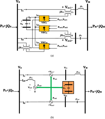
In case of faults occurring on transmission lines, distance relays protect the faulty line by estimating the impedance of the fault location matching it with the set zoning of the relay itself, and issuing a command to disconnect the breakers at the beginning of the line according to the timing defined for them. The projected equations of the distance relays are established using the symmetrical components of the current and voltage measured by the protective CT and CVT connected to the relay and the line parameters under protection. In these studies, UIPC equipment is considered in the middle of the line. This equipment is placed in series–parallel in a transmission line, and it includes two series VSCs in the line in terms of topology, which are installed in parallel, and also includes a parallel VSC linked to the common bus of the two series converters.
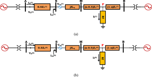
Therefore, according to the mentioned topology, if the distance protection equations of the desired line are planned, the effect of the series and parallel converters of the UIPC equipment will be included in the equations of the distance protection plan and cause deviations in estimating the impedance of the fault location. This aspect has not been addressed in any previous studies on this problem. Reference [19] is the sole article addressing the impact of UIPC on distance protection, highlighting solely the detrimental effects of this equipment on the formulation of distance relays without proposing a solution to this issue. In light of the issues associated with power transmission in power system operations, the utilization of FACTS devices is progressively rising. Their utilization and enhancement of network flexibility are the most viable solutions for addressing the power management issue in the power network. This study proposes the utilization of an phasor estimator for UIPC converters to address the challenges associated with distance relay protection in lines equipped with UIPC.
1.4 Contributions and Novelty
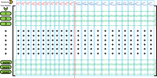
In this article, a scheme for estimating the sequence current and voltage phasor of 72-pulse UIPC voltage source converters at the time of short-circuit fault in transmission lines is presented. Among the prominent points of the proposed design is that there is no need to design and update the new formulation of the distance relay and it can work with the same initial format and the unknown parameters are considered as input. The approach suggested in this research adopts artificial neural network trained to estimate phasors. To implement this model, different scenarios of short circuits in the transmission lines on both sides of the UIPC have been used for different locations, in different phases, for different resistances, and at different times. The input data of this network are in the form of 12 vectors, and these 12 inputs include the size and phase angle of the symmetrical components of voltage and current of all three phases measured by the relay. The output data is a 12 vector, which includes the size and phasor angle of the symmetrical current and voltage components of all three phases of a series voltage source equivalent circuit and a parallel current source equivalent circuit. A total of 3660 fault scenarios have been used for FFN training and modeling in this article. Network modeling under study is implemented in Simulink/MATLAB software and the desired network program is coded in a MATLAB M-file.
- Presenting a method for estimating positive, negative, and zero sequence phasors based on artificial neural network for UIPC voltage and current converters.
- Solving the challenge of distance protection of lines equipped with UIPC without the need for changes in the distance relay formulation.
- Extracting a short circuit analysis model to identify UIPC behavior during a short circuit fault.
- The proposed method is independent of data from both sides of the line and uses current and voltage of one terminal.
- The proposed method is independent of UIPC operating mode and its installation location in the line.
- The proposed method is expandable for different network structures without the need for specific predetermined settings.
1.5 Paper Organization
This article comprises seven general sections. The UIPC-based system is elucidated in Section 2. Section 3 examines and evaluates the impact of UIPC on the distance relay formulation. In Section 4, the theory of the proposed method is defined in three subsets. This section initially introduces the network under investigation, subsequently derives the artificial neural network model for phasor estimation, and concludes with a flowchart of the proposed methodology. Section 5 presents the testing and evaluation of various fault scenarios. Section 6 presents the results of the comparison of the suggested method utilizing two solvers, while Section 7 provides the article's conclusion.
2 Introducing the Basic UIPC

3 Investigating the Impact of UIPC on Distance Relay Formulation
- LG fault

- LL and LLG faults
4 The Proposed Method
4.1 Introducing the Network Under Study
| Networks A and B characteristics | |||||
|---|---|---|---|---|---|
| 230 kV | Base voltage | 60 Hz | Frequency | 230 kV | Line voltage (rms) |
| 7 | X/R ratio | 900 MW | Short-circuit voltage level | (20, −6.8) degree | (A, B) phase angle |
| Characteristics of TL1 and TL2 lines | |||||
|---|---|---|---|---|---|
| 60 Hz | Frequency | 200 km | Length | ||
| 03864 Ω/km | Resistance r0 | 0.0529 Ω/km | Resistance r1 | ||
| 4.1267 × 10⁻³ H/km | Inductance l0 | 0.0014 H/km | Inductance l1 | ||
| 7.751 × 10⁻⁹ F/km | Capacitance c0 | 8.7751 × 10⁻⁹ F/km | Capacitance c1 | ||
| Data for control coefficients of UIPC converters | |||||
|---|---|---|---|---|---|
| Shunt converter | |||||
| 12 | Kp coefficient of voltage controller | 500 | Ki coefficient of voltage controller | ||
| 1 | Kp coefficient of current controller | 5 | Ki coefficient of current controller | ||
| Series converter | |||||
| 1 | Kp coefficient of the controller | 10 | Ki coefficient of the controller | ||
4.2 Extracting the Model of an Artificial Neural Network for Phasor Estimation
4.2.1 Data Normalization and Division
After normalizing the data, they are divided into three sets: 80% for neural network training, 10% for validation, and 10% for testing. The training data are used to train the neural network. 10% of the total data are used to validate the performance of the neural network. This data are used to evaluate the performance of the model during training. With the help of these data, the model is optimized and overfitting is prevented. Validation data helps the model make better parameter settings by checking performance on data not used in direct training. The remaining 10% of the total data is used for model testing. The purpose of this step is to check the performance of the model on data not used in training and validation. These data are used to check the generalizability of the model on new data that were not used in the training and validation stages.
4.2.2 ANN Implementation and Model Extraction
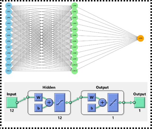
After training the desired FFN network model, information about its settings for software and hardware implementation is obtained. The desired network information obtained in this article is given in Table 2. Using this information, it is possible to implement the desired FFN without the need for training and test data information.
| Code written in MATLAB | ||
|---|---|---|
| Parameter | Description | Value |
| Data loading | The data contains 3660 rows including samples and 24 columns, the first 12 columns are the features and the remaining 12 columns are labels, i.e. outputs | AA = 3660 × 24 |
| Data normalization | Data normalization formula (data normalization to the range [−1,1]) | ((AA—min(AA))./(max(AA)—min (AA))) × 2–1 |
| Data dimensions for neural network | In each step, only one label (output) is estimated according to the input |
Inputs =3660 × 12 Outputs = 3660 × 1 |
| Network creation function | The function is used to create the network | Fitnet (hiddenLayerSize) |
| Input layer | The primary layer that receives the input data | Number of input layers = 1 |
| Input neurons | The number of input neurons (equal to the number of features) | 12 |
| Hidden layers | Intermediate layers between input and output layers | Number of hidden layers =1 |
| Hidden layer activation function | Hyperbolic tangent (tansing) | disp ([‘Hidden Layer Activation Function:’, net. layers {1}. transferFcn]) |
| Hidden layer neurons | The number of hidden layer neurons | 12 |
| Output neurons | The number of output neurons | 1 |
| Output layer activator function | Pureline | disp ([‘Output Layer Activation Function:’, net. layers {2}. transferFcn]) |
| Input preprocessing functions | Preprocessing functions for inputs | {‘removeconstantrows’, ‘mapminmax’} |
| Output preprocessing functions | Preprocessing functions for outputs | {‘removeconstantrows’, ‘mapminmax’} |
| Data division function | All data divider function | ‘dividerand’ |
| Data sharing mode | All data divider mode | ‘sample’ |
| Training data ratio | Proportion of data allocated to training | 80% |
| Validation data ratio | Proportion of data allocated to validation | 10% |
| Test data ratios | Proportion of data allocated to testing | 10% |
| Training function | The function used to train the network (Levenberg–Marquardt) | ‘trainlm’ |
| Performance function | Network performance function | ‘mse’ |
| Graph drawing functions | Functions used to draw performance analysis graphs | {‘plotperform’, ‘ploterrhist’, ‘plotfit’, ‘plotregression’} |
| Network save file | The name of the saved file of the trained network | fitnet.mat |
| Outputs return formula | Formula to restore outputs from normalized state to original values | (((outputs +1)/2) × (max (AA (: 13)) − min (AA (: 13)))) + min (AA (: 13)) |
| Error and performance | Formula for calculating errors and network performance | gsubtract (targets_new, outputs_new), perform (net, targets_new, outputs_new) |
4.2.3 Output Results of the Suggested Model
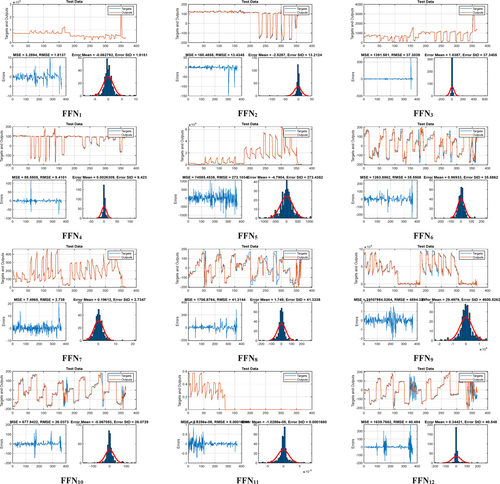
Table 3 tabulates the information on the results of the FFN training and testing for all 12 intended outputs.
| Results | Iteration | Time | Performance | Gradient | Error | Validation |
|---|---|---|---|---|---|---|
| 1000 | 0:00:17 | 2.58e-10 | 3.77e-6 | e-8 | 0 | |
| 134 | 0:00:02 | 0.00373 | 0.0174 | e-5 | 6 | |
| 594 | 0:00:09 | 1.81e-5 | 0.000123 | e-7 | 6 | |
| 52 | 0:00:01 | 0.00160 | 0.00676 | e-5 | 6 | |
| 256 | 0:00:04 | 5.86e-5 | 0.000556 | e-7 | 6 | |
| 48 | 0:00:01 | 0.0306 | 0.0138 | 0.000100 | 6 | |
| 490 | 0:00:08 | 8.49e-5 | 0.000950 | e-8 | 6 | |
| 41 | 0:00:01 | 0.0292 | 0.0223 | e-5 | 6 | |
| 39 | 0:00:01 | 0.00814 | 0.00329 | e-5 | 6 | |
| 36 | 0:00:01 | 0.0253 | 0.0309 | 0.000100 | 6 | |
| 1000 | 0:00:15 | 2.43e-7 | 4.31e-7 | e-8 | 6 | |
| 21 | 0:00:00 | 0.0559 | 0.123 | e-6 | 6 |
4.3 Final Flowchart of the Proposed Method
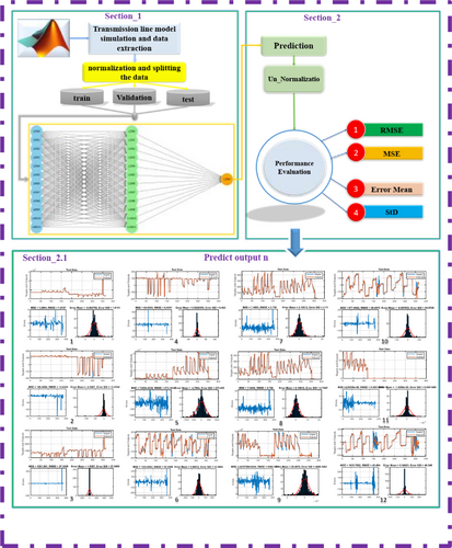
Figure 9 displays the complete flowchart of FFN training steps. Based on the provided flowchart, all training and testing steps as well as output results for 12 parameters are given.
5 Testing and Evaluation of Various Fault Scenarios
5.1 Evaluation of Usual Fault Scenarios
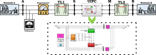
In this part, the goal is to test and evaluate the designed algorithm in a simulated network. For implementation, the network presented in Figure 5 has been used. To test and evaluate the proposed algorithm, 10 different scenarios have been used. To ensure the performance of this proposed plan, these 10 scenarios considered in the neural network training and testing database have not been included. The results presented in Table 4, fault scenarios, show the values recorded by the PMUs at the bus A location. As can be seen in the table, the measured values in bus A are given as the input of the proposed model and the estimation results for 12 output parameters of the model, which include the magnitude and angle of voltage and current of the UIPC converters, are calculated. Each parameter's estimation error is also shown. As can be seen, the accuracy of the proposed estimation method is very suitable at the time of occurrence of any type of short-circuit fault with a variety of changeable parameters. The proposed method in this paper, for the first time, uses the idea of estimating the parameters of the FACTS devices to solve the distance relay challenge. The method includes an expandable compensator for various types of networks.
| Scenario No. | Results of implementation of scenarios | |
|---|---|---|
| 1 | Scenario def. | This scenario assumes that an AG fault with a fault resistance of 15 Ω has occurred at a distance of 40 km from terminal A |
| Input vector | A = [154847.03, 17976.43, 18881.03, 10.68, −177.01, −172.29, 1726.04, 541.23, 897.55, −47.73, −42.39, −49.42] | |
| Estimation results | B = [74767.419, 2730.000, 75822.71, 120.83, 147.18, −158.29, 604.951, 147.510, 0.490, 105.00, −75.33, −23.25] | |
| Estimation error percentage | E = [0.0092, 0.0562, 0.0089, 0.066, 0.089, 0.092, 0.0723, 0.0886, 0.120, 0.099, 0.1442, 0.096] | |
| 2 | Scenario def. | This scenario assumes that a CG fault with a fault resistance of 5 Ω has occurred at a distance of 80 km from terminal A |
| Input vector | A = [164656.46, 8461.79, 12396.65, 11.44, 41.27, −71.59, 1458.86, 254.76, 584.88, −52.82, 176.39, 51.44] | |
| Estimation results | B = [71679.30, 1289.75, 86605.34, 121.74, 36.66, −55.35, 681.10, 134.42, 0.56224, 104.11, 152.63, 79.82] | |
| Estimation error percentage | E = [0.0112, 0.0421, 0.012, 0.032, 0.0901, 0.073, 0.152, 0.168, 0.163, 0.142, 0.1332, 0.165] | |
| 3 | Scenario def. | This scenario assumes that a BCG fault with a fault resistance of 50 Ω has occurred at a distance of 60 km from terminal A |
| Input vector | A = [152893.05, 14984.24, 8730.49, 7.55, 31.86, 12.04, 1745.51, 456.51, 417.06, −39.27, 167.21, 135.22] | |
| Estimation results | B = [75659.47, 2244.14, 48109.66, 119.11, 28.09, 27.38, 466.65, 168.38, 0.314, 96.120, 129.65, 162.570] | |
| Estimation error percentage | E = [0.01321, 0.0925, 0.025, 0.063, 0.192, 0.088, 0.09, 0.0992, 0.220, 0.112, 0.1548, 0.0832] | |
| 4 | Scenario def. | This scenario assumes that an AB fault with a fault resistance of 1 Ω has occurred at a distance of 75 km from terminal A |
| Input vector | A = [147521.59, 33532.99, 0.50, 14.91, −139.39, 176.730, 2060.14, 1023.83, 0.021, −54.91, −4.170, −60.360] | |
| Estimation results | B = [93652.07, 13579.86, 3.33, 126.38, 176.97, −167.20, 240.73, 457.71, 0.000021, −125.54, −38.94, 32.17] | |
| Estimation error percentage | E = [0.0096, 0.0355, 0.0102, 0.068, 0.0889, 0.0958, 0.156, 0.099, 0.133, 0.123, 0.1021, 0.088] | |
| 5 | Scenario def. | This scenario assumes that an ABCG fault with a fault resistance of 20 Ω has occurred at a distance of 20 km from terminal A |
| Input vector | A = [90713.88, 172.26, 0, −4.84, −6.006, −46.65, 3721.23, 6.50, 0, −29.380, −146.210, 79.260] | |
| Estimation results | B = [85631.79, 2592.99, 0, 116.76, 165.81, −74.58, 154.72, 48.17, 0, −105.13, 45.05, 78.99] | |
| Estimation error percentage | E = [0.0086, 0.0525, 0.0111, 0.096, 0.0919, 0.0863, 0.0956, 0.159, 0.023, 0.093 0.09021, 0.126] | |
| 6 | Scenario def. | This scenario assumes that a BG fault with a fault resistance of 15 Ω has occurred at a distance of 120 km from terminal A |
| Input vector | A = [167490.45, 3764.010, 23.330, 11.410, −142.230, 65.55, 1378.25, 114.180, 1.104, −5.40, −5.540, −171.590] | |
| Estimation results | B = [51845.23, 23189.66, 82921.67, 110.96, 90.52, −126.04, 0.1015.77, 256.3, 0.0011, 98.36, 132.42, −138.45] | |
| Estimation error percentage | E = [0.322, 0.424, 0.1265, 0.135, 0.126, 0.266, 0.356, 0.115, 0.253, 0.136, 0.3021, 0.353] | |
| 7 | Scenario def. | This scenario assumes that a BCG fault with a fault resistance of 20 Ω has occurred at a distance of 140 km from terminal A |
| Input vector | A = [161728.62, 5250.51, 16.930, 12.920, −31.41, −7.030, 1588.08, 161.80, 0.80, −56.170, 102.860, 115.730] | |
| Estimation results | B = [45571.83, 23330.03, 60169.30, 92.35, 152.32, 161.20, 858.64, 416.27, 0.00084, 96.85, 142.05, 140.27] | |
| Estimation error percentage | E = [0.3045, 0.224, 0.230, 0.423, 0.223, 0.246, 0.565, 0.0923, 0.355, 0.255, 0.436, 0.429] | |
| 8 | Scenario def. | This scenario assumes that an AC fault with a fault resistance of 1 Ω has occurred at a distance of 170 km from terminal A |
| Input vector | A = [159975.91, 16087.98, 0.00045, 10.22, 83.76, −73.64, 1556.88, 485.62, 0, −47.041, −139.16, 56.36] | |
| Estimation results | B = [32333.610, 54744.190, 2.06, −163.69, −119.88, 95.452, 220.58, 300.081, 0, 77.811, −29.570, 83.601] | |
| Estimation error percentage | E = [0.236, 0.199, 0.159, 0.255, 0.355 0.3, 0.333, 0.463, 0.523, 0.238, 0.3926, 0.442] | |
| 9 | Scenario def. | This scenario assumes that an AB fault with a fault resistance of 100 Ω has occurred at a distance of 110 km from terminal A |
| Input vector | A = [166385.26, 003476.74, 0.001, 10.57, −165.39, −161.89, 1388.14, 108.097, 0, −50.64, −27.97, −58.51] | |
| Estimation results | B = [602787.37, 24784.90, 4.530, 108.32, 65.820, −14.18, 997.590, 283.79, 0, 95.0550, 102.18, −51.320] | |
| Estimation error percentage | E = [0.233, 0.463, 0.333, 0.215, 0.302, 0.365, 0.225, 0.225, 0.115, 0.265, 0.4365, 0.223] | |
| 10 | Scenario def. | This scenario assumes that an ABC fault with a fault resistance of 1 Ω has occurred at a distance of 150 km from terminal A |
| Input vector | A = [200150.004, 725.57, 0, −8.40, −43.48, −64.27, 1805.22, 84.510, 0, 34.0078, −25.74, 35.570] | |
| Estimation results | B = [245341.089, 3480.209, 0, −44.69, 32.13, −59.85, 3250.78, 106.108, 0, −60.80, 9.45, 135.85] | |
| Estimation error percentage | E = [0.232, 0.223, 0.326, 0.4425, 0.105, 0.321, 0.336, 0.256, 0.266, 0.365, 0.265, 0.449] | |
5.2 Sensitivity Analysis
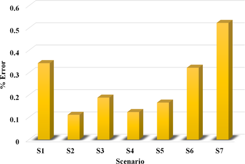
In this part, the goal is to investigate the sensitivity of the suggested algorithm to seven critical scenarios. The conditions of these seven scenarios are given in Table 5. The estimation error results of 12 output parameters are listed in this table. Figure 10 shows the estimation error of ±0 sequence voltage and current phasors of UIPC's converters for seven error scenarios. According to the obtained results, the average parameter estimation error for scenarios S2 and S7 are the lowest and highest values of this sensitivity analysis, respectively. As can be seen, the proposed method can be developed with very good accuracy in various critical conditions because it uses FFN and does not require special adjustments. The robustness of the proposed method with respect to the proposed sensitivities indicates the successful performance of the proposed method.
| Scenario No. | Results of implementation of scenarios | |
|---|---|---|
| S1 | Scenario def. | This scenario assumes that an AB fault with a fault resistance of 500 Ω has occurred at a distance of 150 km from terminal A |
| Estimation error percentage | E = [0.356, 0.365, 0.365, 0.226, 0.269, 0.336, 0.442, 0.1252, 0.330, 0.4589, 0.4442, 0.396] | |
| S2 | Scenario def. | In this scenario, it is assumed that there is a 10% change in the positive and zero sequence impedance of the transmission line in terms of magnitude and angle. In this case, an AB fault with a resistance value of 20 Ω has occurred at a distance of 110 km from terminal A |
| Estimation error percentage | E = [0.0223, 0.0321, 0.026, 0.043, 0.0881, 0.0663, 0.265, 0.139, 0.166, 0.0988, 0.163, 0.223] | |
| S3 | Scenario def. | In this scenario, it is assumed that the UIPC location will be 50 km closer to Terminal A. In this case, a BCG fault with a resistance value of 1 Ω has occurred at a distance of 100 km from terminal A |
| Estimation error percentage | E = [0.0215, 0.112, 0.1450, 0.086, 0.256, 0.265, 0.177, 0.265, 0.336, 0.156, 0.235, 0.202] | |
| S4 | Scenario def. | This scenario assumes that reference active and reactive power injection by the UIPC has been increased by 5%. In this case, a BG fault with a fault resistance of 10 Ω has occurred at a distance of 50 km from terminal A |
| Estimation error percentage | E = [0.0123, 0.0445, 0.0896, 0.122, 0.0969, 0.1258, 0.2056, 0.112, 0.163, 0.139, 0.2121, 0.158] | |
| S5 | Scenario def. | This scenario assumes that the voltage and current signal sampling frequency will deviate (decrease) by 5%. In this case, an ABCG fault with a resistance value of 1 Ω occurs at a distance of 110 km from terminal A |
| Estimation error percentage | E = [0.0625, 0.0776, 0.0866, 0.076, 0.232, 0.0996, 0.225, 0.269, 0.225, 0.365 0.115, 0.156] | |
| S6 | Scenario def. | The scenario assumes that the total length of the transmission line is extended by 20% on both sides of the UIPC. In this case, an AG fault with a resistance value of 100 Ω has occurred at a distance of 200 km from terminal A |
| Estimation error percentage | E = [0.422, 0.369, 0.226, 0.0965, 0.166, 0.368, 0.498, 0.265, 0.336, 0.268, 0.449, 0.401] | |
| S7 | Scenario def. | In this scenario, it is assumed that a Gaussian noise of 20 dB has been injected into the current and voltage samples. In this case, a BC fault with a resistance value of 10 Ω has occurred at a distance of 50 km from terminal A |
| Estimation error percentage | E = [0.665, 0.769, 0.669, 0.3365, 0.429, 0.368, 0.552, 0.3401, 0.448, 0.652, 0.551, 0.499] | |
6 Discussion and Comparison of Results
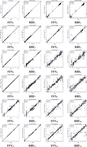
The performance of FFN is contrasted to that of other neural networks in this section of the paper. RBF has been employed for comparison purposes with other neural networks. In general, feedforward neural networks outperform many more complex problems due to their high power and basic structure, which enable them to learn complex nonlinear relationships between input and output. Conversely, RBF neural networks are more appropriate for issues involving linear or quasi-linear relationships as a result of the utilization of radial basis functions. Table 6 and Figure 11 illustrate the results of this assessment. The sole graphical representation of the R index is depicted in the figure. Nevertheless, Table 6 presents the quantitative analysis of the R index, RMSE, and MSE results. Each graph for the R index comprises circular data points, a fitting line, and a two-dimensional regression graph, as illustrated in Figure 11. The regression diagrams for FFN and RBF are 1 and 0.99871, respectively. A FNN value of 1 indicates a perfect correlation between the predicted and actual values. The test data demonstrates that the FFN has a faultless prediction accuracy. Subsequently, the results of output 1 for both neural networks were examined in accordance with the findings in Table 6 in order to conduct a more thorough analysis. The MSE, RMSE, and R values for FNN are 3.289, 1.7137, and 1, respectively, while for RBF, they are 1145921.573, 1070.47, and 0.99871, respectively. The MSE and RMSE indicators are defined to indicate the amount of model error. Consequently, the present model is more accurate when these values are lower, which in this case indicates the optimal performance accuracy of FNN in comparison to RBF. Conversely, the R index's definition permits the assessment of the model's alignment with actual data. The results indicate that both networks have a high coefficient of determination; however, FFN exhibits superior performance with R = 1 compared to RBF with R = 0.99871. The model's perfect fit to the real data is indicated by a coefficient of determination of 1, while a value of 0.99871 is also very near to 1 but slightly lower than FFN. These findings indicate that FFN is capable of a more accurate prediction and a more comprehensive modeling of the data. In general, the FFN network is a superior option for prediction due to its superior agreement with the actual data and reduced error.
| ANN type | Output n prediction | MSE | RMSE | R |
|---|---|---|---|---|
| FFN | 1 | 3.289 | 1.8137 | 1 |
| RBF | 1 | 1145921.573 | 1070.47 | 0.99871 |
| FFN | 2 | 180.48 | 13.43 | 0.98925 |
| RBF | 2 | 519.0411 | 22.78 | 0.96203 |
| FFN | 3 | 1391.581 | 37.3039 | 0.99687 |
| RBF | 3 | 4338.73 | 58.67 | 0.9919 |
| FFN | 4 | 88.5505 | 9.4101 | 0.99 |
| RBF | 4 | 332.813 | 18.24 | 0.97093 |
| FFN | 5 | 74585.4538 | 273.103 | 0.99984 |
| RBF | 5 | 5327533.1092 | 2308.1449 | 0.98835 |
| FFN | 6 | 1263.856 | 35.5508 | 0.94813 |
| RBF | 6 | 1936.2029 | 44.0023 | 0.92179 |
| FFN | 7 | 7.4965 | 2.738 | 0.99968 |
| RBF | 7 | 656.376 | 25.619 | 0.97477 |
| FFN | 8 | 1706.8764 | 41.3144 | 0.91694 |
| RBF | 8 | 1740.1514 | 41.7151 | 0.90791 |
| FFN | 9 | 21107884.026 | 4594.33 | 0.98958 |
| RBF | 9 | 50168648.4053 | 7082.983 | 0.97437 |
| FFN | 10 | 677.9422 | 26.0373 | 0.96726 |
| RBF | 10 | 1257.1503 | 35.4563 | 0.94223 |
| FFN | 11 | 2.8256e-8 | 0.00016 | 1 |
| RBF | 11 | 0.00011396 | 0.010675 | 0.99792 |
| FFN | 12 | 1639.7661 | 40.494 | 0.9176 |
| RBF | 12 | 2231.2762 | 47.2364 | 0.89547 |
7 Conclusion
- Presenting a new method to solve the challenge of formulating distance relays during short-circuit faults in UIPC-compensated transmission lines;
- The method developed in this paper can be applied as an input into the distance relay equations and there is no need to update the relay equations;
- The proposed method is based on a training-based model. The data required to generate the estimation model is trained based on the implementation of different fault scenarios for various locations, times, phases, and with different resistances;
- The solver of the proposed method is based on FFN, which makes training, learning, and model extraction very easy and simple;
- According to the results of implementing different scenarios and also the results presented in the sensitivity analysis, the proposed method is very robust to different parameters and to critical conditions;
- The proposed method is not dependent on the data of both line terminals and only uses the phasor data of one line terminal during the fault.
Nomenclature
-
- aj/bj
-
- the coefficient used in the linear equation of the neural network
-
- ē
-
- mean error
-
- fSE2
-
- voltage frequency of series converter 2
-
- fshunt
-
- voltage frequency of shunt converter
-
- KI
-
- integrator control coefficient
-
- KP
-
- proportional control coefficient
-
- n
-
- the total number of samples
-
- Wkj
-
- the weight coefficient of the neural network
-
- x
-
- input variable of the neural network
-
- Xnormalization
-
- normalized variable for neural network training
-
- y
-
- the variable related to the neural network
-
- zj
-
- exponential variable of the neural network
-
- I*d
-
- calculated reference current for d-axis
-
- I*q
-
- calculated reference current for q-axis
-
- I1
-
- inductive branch current of the UIPC
-
- I2
-
- capacitive branch current of the UIPC
-
- Iabc_SE1
-
- three-phase current flowing through series converter 1
-
- Iabc_SE2
-
- three-phase current flowing through series converter 2
-
- Iabc_shunt
-
- three-phase current flowing through the parallel converter
-
- id
-
- instantaneous current of d-axis
-
- Id
-
- reference current of d-axis
-
- Īd
-
- average current of d-axis
-
- id1
-
- injected current of dc-link of series converter 1
-
- id2
-
- injected current of dc-link of series converter 2
-
- id3
-
- injected current of dc-link of shunt converter
-
- If
-
- injected current at the fault point
-
- Iq
-
- reference current of q-axis
-
- Īq
-
- average current of q-axis
-
- IR
-
- current measured at the relay location
-
- IS(0)
-
- zero-sequence current of terminal S
-
- IS(1)
-
- positive-sequence current of terminal S
-
- IS(2)
-
- negative-sequence current of terminal S
-
- Ish
-
- current of the shunt converter of the UIPC
-
- IUIPC(0)
-
- zero-sequence current of shunt converter of the UIPC
-
- IUIPC(1)
-
- positive-sequence current of shunt converter of the UIPC
-
- IUIPC(2)
-
- negative-sequence current of shunt converter of the UIPC
-
- Vabc_shunt
-
- three-phase voltage of shunt converter
-
- Vd
-
- d-axis voltage in UIPC control system
-
-
- calculated d-axis voltage in UIPC control system
-
-
- average d-axis voltage in UIPC control system
-
- VDC
-
- DC-link voltage
-
- VLabc_SE2
-
- three-phase voltage on the left-side link of the series converter 2
-
- Vmse
-
- the voltage value measured at the connection point of the shunt converter
-
- Vq
-
- q-axis voltage in UIPC control system
-
- q
-
- calculated q-axis voltage in UIPC control system
-
- q
-
- average q-axis voltage in UIPC control system
-
- VRabc_SE1
-
- three-phase voltage on the right-side link of the series converter 1
-
- VRabc_SE2
-
- three-phase voltage on the right-side link of the series converter 2
-
- Vref
-
- reference voltage of the bus connected to the shunt converter
-
- VS
-
- voltage of bus S
-
- VM
-
- voltage of bus M
-
- VS(0)
-
- zero-sequence voltage of bus S
-
- VS(1)
-
- positive-sequence voltage of bus S
-
- VS(2)
-
- negative-sequence voltage of bus S
-
- Vse1
-
- injected voltage of converter 1
-
- Veq(1)
-
- the positive-sequence voltage of the equivalent Thevenin circuit of converter 1
-
- Veq(0)
-
- the zero-sequence voltage of the equivalent Thevenin circuit of converter 2
-
- Vse2
-
- injected voltage of converter 2
-
- Vse3
-
- injected voltage of converter 3
-
- Vsek
-
- voltage of the series converter
-
- VUIPC(0)
-
- zero-sequence voltage of series converter of the UIPC
-
- VUIPC (1)
-
- positive-sequence voltage of series converter of the UIPC
-
- VUIPC(2)
-
- negative-sequence voltage of series converter of the UIPC
-
- VVL-L
-
- line-to-line voltage set in the control system
-
- Pex1
-
- active output power of converter 1
-
- Pex2
-
- active output power of converter 2
-
- Pex3
-
- active output power of converter 3
-
- Pmi
-
- amplitude modulation
-
- Pmi1
-
- amplitude modulation of converter 1
-
- Pmi2
-
- amplitude modulation of converter 2
-
- Pmi3
-
- amplitude modulation of converter 3
-
- Pmr
-
- phase modulation
-
- Pmr1
-
- phase modulation of converter 1
-
- Pmr2
-
- phase modulation of converter 2
-
- Pmr3
-
- phase modulation of converter 3
-
- PM
-
- the active power of bus M
-
- PS
-
- the active power of bus S
-
- PSE1REF
-
- reference active power of series converter 1
-
- PSE2REF
-
- reference active power of series converter 2
-
- QM
-
- reactive power bus M
-
- QS
-
- reactive power bus S
-
- QSE1REF
-
- reference reactive power of series converter 1
-
- QSE2REF
-
- reference reactive power of series converter 2
-
- Bsh
-
- equivalent susceptance of the shunt converter
-
- Beq
-
- equivalent susceptance of the series converter
-
- Xl
-
- reactance of the inductive branch
-
- Xc
-
- reactance of the capacitive branch
-
- Xeq
-
- reactance from the fault location to the relay location
-
- Xeq1
-
- equivalent reactance of series converter 1
-
- Xeq2
-
- equivalent reactance of series converter 2
-
- Xsh
-
- equivalent reactance of the shunt converter
-
- Xsh
-
- reactance of the transformer
-
- XT1
-
- reactance of the transformer in series with converter 1
-
- XT2
-
- reactance of the transformer in series with converter 2
-
- XT3
-
- reactance of the transformer of the shunt converter
-
- Z1
-
- impedance of the protected line
-
- Z1(0)
-
- zero-sequence impedance from the relay location to the fault location
-
- Z1(1)
-
- positive-sequence impedance from the relay location to the fault location
-
- ZR
-
- the impedance calculated from the relay location to the fault location
-
- Rf
-
- fault resistance
-
- αIs(0)
-
- angle of the zero-sequence current of terminal S (degree)
-
- αIs(1)
-
- angle of the positive-sequence current of terminal S (degree)
-
- αIs(2)
-
- angle of the negative-sequence current of terminal S (degree)
-
- αIUIPC(0)
-
- zero-sequence current of UIPC's shunt converter (degree)
-
- αIUIPC(1)
-
- positive-sequence current of UIPC's shunt converter (degree)
-
- αIUIPC(2)
-
- negative-sequence current of UIPC's shunt converter (degree)
-
- αVs(0)
-
- zero-sequence voltage angle of terminal S (degree)
-
- αVs(1)
-
- positive-sequence voltage angle of terminal S (degree)
-
- αVs(2)
-
- negative-sequence voltage angle of terminal S (degree)
-
- αVUIPC(0)
-
- zero-sequence voltage angle of the UIPC's shunt converter (degree)
-
- αVUIPC(1)
-
- positive-sequence voltage angle of the UIPC's shunt converter (degree)
-
- αVUIPC(2)
-
- negative-sequence voltage angle of the UIPC's shunt converter (degree)
-
- δSM
-
- voltage angle difference between buses S and M
-
- θSE2
-
- voltage angle calculated in the control system of the voltage converter series 2
-
- θshunt
-
- voltage angle of the UIPC's shunt converter
-
- φ1
-
- phase-shift angle of the voltage of series converter 1
-
- φ2
-
- phase-shift angle of the voltage of series converter 2
-
- φM
-
- voltage angle of terminal M
-
- φS
-
- voltage angle of terminal S
Author Contributions
Babak Bahadori: investigation, writing – original draft, software, formal analysis, data curation, resources. Ali Nahavandi: project administration, supervision, writing – review and editing, methodology. Mahyar Abasi: conceptualization, writing – review and editing, methodology, supervision, project administration, validation.
Conflicts of Interest
The authors declare no conflicts of interest.
Open Research
Data Availability Statement
Research data are not shared.


