Data-driven probabilistic curvature capacity modeling of circular RC columns facilitating seismic fragility analyses of highway bridges
Abstract
The availability of reliable probabilistic capacity models of reinforced concrete (RC) columns is a cornerstone for high-confidence seismic fragility and risk analyses of highway bridges. Existing studies often perform physics-based pushover or moment–curvature analyses for the capacity modeling of RC columns, which may encounter nonconvergent problems under high levels of nonlinearities in structural material constitutive models and elements, and become computationally inefficient especially when the analysis model contains plenty of cases involving multisource uncertainties. To mitigate the nonconvergent issues as well as release the computational burden of RC column capacity estimates, this study explores the potency of artificial neural network for data-driven probabilistic curvature capacity modeling of circular RC columns, which can facilitate seismic fragility assessment of highway bridges. To this end, a large database is developed by fiber-section-based moment–curvature analyses covering major ranges of concrete and steel strengths, reinforcement ratios, vertical loads, and geometries of RC columns in engineering practices. To obtain an accurate data-driven model, a fivefold cross-validation training and test process is performed to optimize the neural network architecture. The optimized neural network leads to a reliable data-driven model for estimating multilevel curvature capacity indices with percentage errors less than 15%. Finally, a typical highway bridge is taken as a case study to demonstrate the applicability of the developed data-driven capacity model for the expediency of seismic fragility analysis. For ease of implementation, the database and associated codes are available at https://bit.ly/3A1dh1V.
1 INTRODUCTION
The seismic fragility analysis is a paramount component across the pipeline of performance-based earthquake engineering. The fragility of a structure is commonly defined by the probability of seismic demand exceeding a specific capacity index under a specific seismic intensity measure (IM). Apparently, the capacity index is a keystone for developing reliable fragility curves of structures. Establishing capacity indices (or called damage indices) of RC columns has been a classical research topic in structural earthquake engineering dating back to the 1960s1 and lasted for several decades2-4 till recently,5, 6 across which various indices with different levels of complexity are proposed to account for cumulative ductility damage together with fatigue and local buckling effects. Nevertheless, prevalent studies on bridge seismic fragility analyses, as reviewed and summarized in reference [7], still utilize simple capacity indices of RC columns in the (1) material level such as rebar strains,8, 9 (2) section level such as curvature,10 and (3) component level such as column drift ratio.11 For RC columns involving both rebar and concrete damage under earthquakes, a material-level capacity index relying on either rebar or concrete strain is not adequate to reflect the damage extents of the entire RC column. Instead, section- and component-level capacity indices normally cover the behavior of both rebars and concrete, thereby being better solutions for fragility analyses of RC bridge columns. In that respect, physics-based moment–curvature (M–φ) and pushover analyses are often carried out for multilevel capacity modeling of RC columns.12, 13 However, such physics-based analyses often meet nonconvergent problems, particularly when high nonlinearities are involved in structural material constitutive models and elements. Also, the physics-based analyses always require high computational costs, especially when the assessed bridge finite element (FE) model contains many cases that represent structural and seismic loading uncertainties. To relieve or mitigate the computationally nonconvergent issues as well as release the computational burden of RC column capacity modeling, data-driven approaches can be an alternative and promising choice. For example, Jadid and Fairbairn14 investigated the role of simple artificial neural network (ANN) architecture (with only one hidden layer) to assist experimental work for estimating yield moment and curvature (i.e., output variables) of a rectangular RC beam section. Caglar et al.15 applied ANN to yield and ultimate curvature estimates of circular RC columns, but the input variables in their ANN model are limited to external vertical loads, column diameter, and longitudinal and transverse reinforcement ratios, while other critical variables such as concrete and rebar strength as well as cover thickness are not considered. Therefore, the application scope of this model is limited. It can be found that existing studies on data-driven curvature capacity modeling are characterized by a limited number of input and output variables, and the data-driven models are not accessible, such that the applicability is generally low, especially for seismic fragility and associated risk and resilience assessment that requires multiple limit states for the sake of accurate performance-based assessment. More importantly, existing studies never address the potency of ANN for uncertainty quantification of capacity indices of RC columns, which is a critical character that affects the shape of fragility curves. Therefore, there are gaps yet to be filled to achieve widely applicable, publicly accessible, and high-confidence data-driven probabilistic multilevel (i.e., different limit states) capacity models for RC columns toward efficient and high-confidence fragility and associated risk and resilience assessment.
To address these research gaps, this study explores the potency of ANN for data-driven probabilistic section-level (i.e., curvature) capacity modeling of circular RC columns that have been the most popular substructure type for highway bridges. Note that data-driven component-level (e.g., drift ratio) capacity models will be studied in the future paper. The developed data-driven model is expected to facilitate seismic fragility assessment of highway bridges. This paper is organized as follows: A database that covers major ranges of column design parameters in engineering practices is first developed via physics-based M–φ analyses based on fiber-section models in OpenSeesPy.16 Then, a data-driven probabilistic curvature capacity model is developed using ANN involving a multifold cross-validation process to identify the optimal ANN architecture for the studied problem. To demonstrate the applicability of the data-driven model, a typical highway bridge is adopted as a case study for seismic fragility analyses using the data-driven and physics-based curvature capacity models for comparisons. Finally, conclusions are addressed, and limitations and future research needs are briefly discussed.
2 DATABASE DEVELOPMENT
2.1 Description of ANN
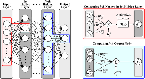
Based on the above description of ANN architecture, N (the number of hidden layers) and Q (the number of neurons in each hidden layer) are apparently two critical parameters for ANN modeling. Larger N and Q indicate a deeper architecture that may better deal with a more complex problem in which the output and input variables have a higher nonlinearity relationship, but meanwhile perhaps meet an overfitting issue. Therefore, an ANN with relatively smaller N and Q that can achieve a reasonable prediction accuracy is preferable for the sake of computational efficiency as well as for overfitting-issue mitigation. In that respect, one of the focuses of this paper is to identify the optimal N and Q for the assessed problem.
2.2 Input variables: Design parameters of RC columns and their sampling
The design of RC columns is mainly dominated by eight parameters taken as the input variables for ANN, including height (H), diameter (D), axial load ratio (α), cover thickness (tc), concrete compressive strength (fc), rebar yield strength (fy), and longitudinal and transverse reinforcement ratios (ρl and ρs, respectively), as illustrated in Figure 2. To create a large database that covers the ranges of these parameters in engineering practices, extensive surveys are conducted by literature reviews as well as communications with experienced bridge engineers. The outcome of these efforts is to consider the column diameter as a scenario parameter from 1.1 to 1.9 m with an interval of 0.2 m, leading to five scenarios listed in Table 1. In each scenario, the rest seven parameters are considered as random variables with specific distribution functions according to existing literature or engineering surveys in this study, as detailed in Table 2. Note that although the column height (H) is not involved in the section M–φ analyses, it is considered in the database for the investigation of RC column failure modes for other scheduled studies. Regarding the database development, the Latin hypercube sampling technique29 is utilized to randomly generate 360 samples for each scenario following the distribution features listed in Table 2, resulting in a database of 1800 samples for ANN modeling. The lower and upper boundaries listed in Table 2 represent the ranges of the randomly generated data set, which also indicate the application scope of the later developed ANN model. Note that due to the relatively small sampling number (i.e., 360) for each scenario, the lower and upper boundaries are not strictly symmetric with respect to the mean values of the normally and uniformly distributed variables. For the expediency of implementation, the created database and associated codes can be accessible at https://bit.ly/3A1dh1V.

| Parameter (unit) | Description | Scenario | Database boundary | |||||
|---|---|---|---|---|---|---|---|---|
| A | B | C | D | E | Lower | Upper | ||
| D (m) | Column diameter | 1.1 | 1.3 | 1.5 | 1.7 | 1.9 | 1.1 | 1.9 |
- Abbreviation: RC, reinforced concrete.
| Parameter (unit) | Description | Distribution | Mean | COV (%) | Source | Boundary of the generated database | |
|---|---|---|---|---|---|---|---|
| Lower | Upper | ||||||
| fc (MPa) | Concrete compressive strength | Normal | 40 | 12 | [26] | 26 | 55 |
| fy (MPa) | Rebar yield strength | Normal | 448 | 8 | [27] | 343 | 549 |
| ρl | Longitudinal reinforcement ratio | Uniform | 0.02 | 29 | [28] | 0.01 | 0.03 |
| ρs | Transverse reinforcement ratio | Uniform | 0.009 | 33 | [28] | 0.004 | 0.013 |
| α | Column axial load ratio | Normal | 0.1 | 20 | [10] | 0.03 | 0.16 |
| H (m) | Column height | Uniform | 9.5 | 33 | This study | 4 | 15 |
| tc (m) | Cover thickness | Uniform | 0.045 | 19 | This study | 0.03 | 0.06 |
- Abbreviation: COV, coefficient of variance.
2.3 Output variables: Multilevel curvature capacity indices of RC columns
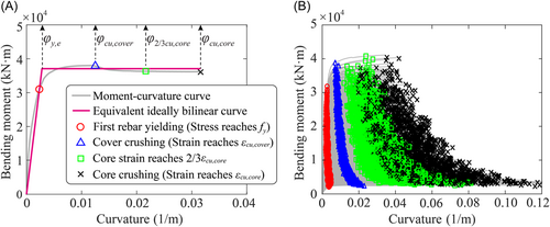
Output variables examined in this study are defined based on the section M–φ relationship,30 as illustrated in Figure 3, including the equivalent yield curvature (φye), cover crushing curvature (φcu, cover), 2/3 core strain-corresponded curvature (φ2/3cu, cover, that is, concrete core strain reaches two-thirds of core crushing strain), and core crushing curvature (φcu, cover). As highlighted in Figure 3A, φye is determined via an ideally bilinear fitting curve, which crosses the first rebar yielding limit state, following the energy-equivalency principle (the same area below the two curves).31 These four capacity indices have been adopted to represent slight, moderate, severe, and complete damage states of RC columns (e.g., references [10, 30, 31]). Figure 3B shows all the 1800 samples' M–φ relationships obtained by physics-based M–φ analyses using fiber-section models in OpenSeesPy.16 More specifically, the longitudinal rebar fibers are modeled using the Steel02 material with a constant elastic modulus of 200 GPa and a postyield hardening ratio of 0.005.32 The concrete fibers are mimicked by the Concrete04 material with the strength-corresponded strain of 0.002 and crushing strain of εcu, cover = 0.004 for the concrete cover,33 while those for the concrete core are determined following Mander et al.,34 which results in the concrete core crushing strain εcu, core accounting for the variable transverse reinforcement ratios. It is worth noting that the concrete strain (e.g., εcu, cover and εcu, core) and the steel elastic modulus and hardening ratio parameters are commonly not the dominant variables in real-world bridge design, thereby they are not taken as input variables in ANN models.
3 DATA-DRIVEN MODEL OPTIMIZATION AND EVALUATION
3.1 Optimization of ANN architecture via multifold cross-validation
To develop a reliable ANN model for high-confidence curvature capacity prediction, the architecture of ANN needs to be optimized in advance. To this end, a k-fold cross-validation is followed, as depicted in Figure 4. More specifically, the input–output database obtained from the above-mentioned M–φ analyses is first normalized for better expediency of ANN modeling, that is, each variable is normalized into a range of [0,1]. The normalized data set is randomly split into a training and test set with a specific ratio such as 70%–30% as adopted in this study. Note that such a ratio is commonly determined by the size of the prepared data set to ensure the relatively small-sized test set contains enough data to generally cover the data ranges of the training set so that the test set can better evaluate the trained model. Using the training set, a k-fold cross-validation training and test process can be performed to identify the optimal parameters for ANN. This study focuses on the number of hidden layers and neurons in ANN. In the cross-validation process, the training set is further split into k folds (e.g., k = 5, a common choice in machine learning applications35 and adopted in the present study), each acts as a test subset in turn to evaluate the trained model based on the rest k − 1 subset. Accordingly, k trials of training and test derive k training errors and k test errors for each ANN parameter examined, such that relationships between the errors and the examined parameter can be plotted to identify the optimal parameter that leads to sufficiently small errors, particularly small test errors that are robust to the k trials. Based on the optimal parameters, the training set is again used to develop the data-driven model, which is further evaluated by the test set.
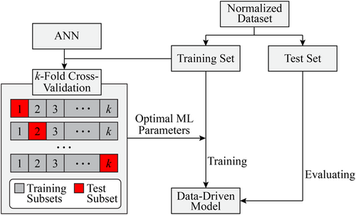
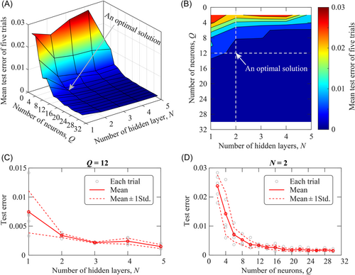
Figure 5 shows the sensitivity of test errors to N and Q in the fivefold cross-validation process. A global inspection of Figure 5A,B indicates that the mean test error of the five trials decreases significantly with the increasing Q until Q = 12 around and then changes very slightly. N is relatively less influential, particularly when N ≥ 2 and Q ≥ 12. Therefore, N = 2 and Q = 12 tend to be an optimal solution that balances the training computational efficiency and model accuracy, although other sets of N and Q such as N = 1 and Q = 16 may also be selected. To confirm this observation, local inspections of the test error sensitivities to N and Q across the identified optimal solution (N = 2 and Q = 12) are shown in Figure 5C,D. Apparently, the five trials in the cross-validation process lead to similar trends that N = 2 and Q = 12 is an optimal solution, that is, corresponding to quite small errors robust to the five trials.
3.2 Evaluation of the developed data-driven model
Based on the identified optimal ANN architecture, that is, two hidden layers each with 12 neurons, data-driven models for multilevel curvature capacity indices are developed. Since an ANN model inherently contains uncertainties in the initial selection of regression and bias constants, 100 runs are conducted and the mean of the outputs of the 100 runs are adopted to demonstrate the performance of the data-driven, as shown in Figure 6 in the form of one-to-one comparisons between the observed and predicted four curvature capacity indices in terms of training and test sets. It is worth noting that the 100 runs cost less than 5 min using an ordinary computer notebook with a Core i5 CPU and 8 GB RAM. In conclusion, the developed data-driven model is expected to well capture multilevel curvature capacity indices of circular RC columns with an error less than 15% in general, as highlighted in Figure 6 using two dashed lines. On the other hand, as fragility analyses often require mean and dispersion values of the curvature capacity indices, Table 3 compares the data-driven predicted and M–φ analysis observed mean and standard deviation of the examined four indices in terms of the training and test sets. From Table 3, the data-driven model accurately predicts the means with almost no errors (less than 2%) and generally captures the standard deviation (errors within 15%), which is commonly acceptable for fragility analyses of bridges. Future studies can expand the database and meanwhile explore more advanced machine learning methods for prediction accuracy improvement.

| Training set | Test set | ||||||||
|---|---|---|---|---|---|---|---|---|---|
| φye | φcu, cover | φ2/3cu, core | φcu, core | φye | φcu, cover | φ2/3cu, core | φcu, core | ||
| Mean (×10−2) | (1) Observed | 0.372 | 1.17 | 3.30 | 4.96 | 0.374 | 1.19 | 3.39 | 5.09 |
| (2) Predicted | 0.372 | 1.16 | 3.29 | 4.94 | 0.374 | 1.17 | 3.34 | 5.01 | |
| |(2) − (1)|/(1) | 0% | 1% | 0% | 0% | 0% | 1% | 2% | 2% | |
| Standard deviation (×10−2) | (3) Observed | 0.0782 | 0.282 | 1.13 | 1.70 | 0.075 | 0.298 | 1.23 | 1.84 |
| (4) Predicted | 0.0745 | 0.254 | 1.03 | 1.56 | 0.072 | 0.255 | 1.09 | 1.65 | |
| |(4) − (3)|/(3) | 5% | 10% | 9% | 8% | 4% | 15% | 11% | 10% | |
- Abbreviation: ANN, artificial neural network.
4 IMPLEMENTATION OF FRAGILITY ANALYSIS OF A HIGHWAY BRIDGE
4.1 Fragility analysis method
4.2 Assessed highway bridge example and numerical modeling
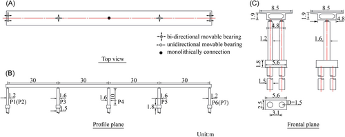
A typical three-span continuous concrete highway overpass bridge in China is taken as the bridge example. Figure 7 describes the geometric configuration of the bridge. The bridge has an overall length of 120 m (4 × 30 m). The deck adopts a box-girder with 8.5 m width and 1.9 m depth. The deck ends are supported by double-column circular cross-section columns with a diameter of 1.2 m, and the interior columns consist of 1.6-m-diameter circular cross-sections. Each column has a total height of 10 m. As shown in Figure 7A, column P4 is monolithically connected to the deck, while spherical steel bearings are installed on other columns to connect the superstructure. The columns are erected on pile-group foundations with two 1.5-m-diameter piles for each footing. The decks are constructed using Chinese Grade C50 concrete26 (axial compressive strength of 32.4 MPa); the columns adopt Chinese Grade C40 concrete (axial compressive strength of 26.8 MPa) and HRB400 reinforcement (tensile strength of 400 MPa), while Chinese Grade C35 concrete (axial compressive strength of 23.4 MPa) is employed for the footings.
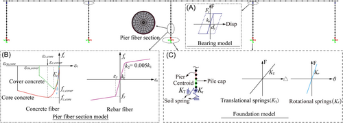
Elastic-perfectly plastic material was adopted to represent the constitutive relationship of the spherical steel bearings (Figure 8A). Nonlinear beam-column fiber elements were used to model the columns (Figure 8B). Concrete04 material was employed to define the stress–strain relationship of unconfined and confined concrete, and the reinforcement fibers were simulated using the Steel02 material. The modeling parameters for the columns of the case study bridge are listed in Table 4. In addition to these parameters, the column axial load ratio (α) is determined by the constant deck mass and the column compressive strength. It is noted that the shear failure pattern was not simulated for columns because the capacity design principle was adopted, and thereby the flexural failure prevails. The pile caps were modeled through the elastic beam-column elements and their masses were imparted to the centroids. The soil-structure interaction was considered as 6-degree-of-freedom linear soil springs (Figure 8C) and their stiffness refers to Mangalathu et al.28 Rayleigh damping with suitable coefficients ( and ) was adopted so that the entire system damping at the frequencies of interest distributes around 5%. Modal analyses were conducted for the bridge example, and the average first natural vibration period is 1.59 s.
| Category | Parameter (unit) | Description | Distribution | Mean | COV (%) | Source |
|---|---|---|---|---|---|---|
| Material strengths | fc (MPa) | Concrete compressive strength | Normal | 40 | 12 | [26] |
| fy (MPa) | Rebar yield strength | Normal | 448 | 8 | [27] | |
| Reinforcement ratios | ρl | Longitudinal reinforcement ratio | Uniform | 0.02 | 29 | [28] |
| ρs | Transverse reinforcement ratio | Uniform | 0.009 | 33 | [28] | |
| Geometries | D (m) | Column diameter | Deterministic | 1.6 | / | / |
| H (m) | Column height | Deterministic | 10 | / | / | |
| tc (m) | Cover thickness | Deterministic | 0.045 | / | / |
- Abbreviations: COV, coefficient of variance; RC, reinforced concrete.
To consider the uncertainty in the ground motion characteristics in the subsequent fragility analysis, a set of 80 unscaled broad-band ground motion records for soil sites of California was selected by Baker et al.42 (Set #1A and Set #1B ground motions in their report) were collected. To expediently validate the efficiency of the data-driven capacity model in the vulnerability assessment, this study solely concentrates on the longitudinal response of the bridge. Therefore, for each ground motion pair, the component with higher shaking intensity was selected and input along the longitudinal bridge direction. Moreover, the curvature at the bottom of the middle column (P4) was selected as the engineering demand parameter for analyses.
4.3 Comparison of data-driven and physics-based curvature capacity indices
Figure 9 compares the physics-based and data-driven multilevel curvature capacity indices obtained from the ANN model and OpenSeesPy fiber-section model, respectively. It is evident that the data-driven model successfully predicts the four capacity indices all with errors less than 15%. Moreover, the means and standard deviations of the data-driven and physics-based results are compared as listed in Table 5, where the errors for the means and standard deviations are less than 3% and 10%, respectively. This level of accuracy is commonly acceptable for engineering fragility analyses. It is expected that quite close fragility curves could be achieved based on the data-driven and physics-based capacity models, as elucidated in the following section.

| φye | φcu, cover | φ2/3cu, core | φcu, core | ||
|---|---|---|---|---|---|
| Mean (×10−2) | (1) Physics-based | 0.339 | 1.06 | 3.01 | 4.51 |
| (2) Data-driven | 0.347 | 1.09 | 3.08 | 4.62 | |
| |(2) − (1)|/(1) | 3% | 2% | 2% | 2% | |
| Standard deviation (×10−2) | (1) Physics-based | 0.0259 | 0.0997 | 0.702 | 1.05 |
| (2) Data-driven | 0.0261 | 0.0905 | 0.765 | 1.16 | |
| |(4) − (3)|/(3) | 1% | 9% | 9% | 10% |
4.4 Comparison of fragility curves using data-driven and physics-based capacity models
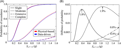
Based on the Cloud method,38 fragility curves of column P4 using physics-based and data-driven curvature capacity models were derived and compared respecting different damage states, as illustrated in Figure 10. Generally, from Figure 10A, fragility curves with the aid of the data-driven capacity models are extremely close to the ones based on the physics-based capacity models for all the damage states. Meanwhile, it can be found that the estimated fragility errors using the data-driven capacity model are smaller for both extensive and complete damage states than the slight and moderate damage states across the assessed IM range. Specifically, Figure 10B depicts the difference between the fragility curves achieved by the two capacity models. The maximum errors for different damage states are 1.8%, 1.9%, 0.8%, and 0.4%, respectively, across the assessed IM range. All errors of less than 2% indicate the effectiveness and applicability of the ANN data-driven RC column capacity model in the fragility analysis and subsequent risk and resilience assessment.
5 CONCLUSIONS
- (1)
The optimized neural network has high computational efficiency, and the resulting data-driven model is adequately reliable to estimate the mean value and standard deviation of the multilevel curvature capacity indices with percentage errors less than 15%.
- (2)
The developed data-driven model has high confidence to predict multilevel curvature capacity indices of RC columns with percentage errors less than 15%.
- (3)
The fragility curves derived based on the data-driven capacity model are exceedingly close to the ones developed using physics-based capacity models, with a maximum difference of less than 2% for all the damage states.
Further studies are needed to expand the database and meanwhile explore more advanced machine learning methods for the prediction accuracy improvement of the data-driven capacity model. Future studies will also explore data-driven component-level (e.g., drift ratio) capacity models. Moreover, the data-driven models are expected to be applied in the risk and resilience assessment of roadway networks.
ACKNOWLEDGMENT
This study is partially supported by the Natural Science Foundation of China (Grant No. 52008155).
CONFLICTS OF INTEREST
The authors declare no conflicts of interest.


