Data-driven analysis of the spatial dependence of grouting efficiency during tunnel excavation
Abstract
Grouting with water–cement mixtures is the most widely used and cost-effective method for managing excess water inflow during tunnel construction. Due to uncertain geological and hydrological conditions, current grouting design relies heavily on the experience of onsite engineers. Recent advances in machine learning offer a promising alternative to traditional design to predict grout volume and improve grouting efficiency. Here, an artificial neural network (ANN) model was developed using the data set from an operation tunnel of Jurong Rock Caverns in Singapore to showcase an efficient and physics-guided training strategy. The ANN model was refined by incorporating the spatial scenarios, including the number of grouting holes in four quadrants of tunneling faces, the sequence of grouting screens along the tunnel axis, and the order of grouting rounds on the tunneling faces. The results indicate that an improved training strategy should encompass the grouting process, from Round 1 with grouting holes uniformly distributed around the tunnel periphery, to Round 2 with grouting holes drilled midway between neighboring first-round holes, and to Round 3 with grouting holes determined by onsite engineers. This model, trained based on the order of grouting rounds, performs better than the other models, highlighting the importance of establishing machine learning models grounded in physical principles. The finding was verified by the data set from another operation tunnel and concluded with a perspective on future grouting research.
Highlights
-
Machine learning aids in enhancing grouting efficiency in tunnel construction.
-
Spatial factors play an important role in machine learning modeling.
-
Training with the grouting process improves the performance of a machine learning model.
1 INTRODUCTION
Grouting with water–cement mixtures is the most common and effective method for controlling water inflow during underground excavation (Kang et al., 2023; Li et al., 2016). The pressurized grout is injected into rock discontinuities to seal water pathways and prevent inflow into the excavation. However, determining the optimal grouting parameters is challenging due to highly variable geological and hydrological factors, such as rock type, joint density, groundwater pressure, and water inflow rate, which can vary substantially from site to site, complicating the grouting design (Corson et al., 2021; Stille & Gustafson, 2010; Tian et al., 2024; Wanniarachchi & Wu, 2021). Currently, no standardized design codes or guidelines specify when the grouting process should stop or how to accurately calculate the required grout volume. As a result, engineers rely heavily on their experience and judgment. This process is often iterative, where initial grouting parameters, such as injection pressure, grout mix ratio, and injection rate, are selected based on prior experience and site-specific conditions. These parameters are then adjusted in real time according to field observations, such as changes in the water inflow rate, grout volume, and ground behavior during the grouting process.
In complex geological environments, such as those with highly jointed rocks or high groundwater pressures, achieving an effective grout seal can be particularly challenging. Engineers may need to conduct multiple grouting rounds or adjust the grout mix and grouting pressure to adapt to changing underground conditions. These challenges highlight the need for more advanced methods to predict grout volume and determine stopping criteria. For example, grout volume is numerically predicted using grout properties and hydrogeological data (Gustafson & Stille, 1996). Estimating the grout spread distance in dilatant rock joints helps enhance the grouting performance, with the deformation limiting curve serving as a stopping reference (Rafi & Stille, 2021). Finite–discrete element modeling simulates the coupled hydro-mechanical processes, revealing the anisotropic grout penetration caused by joint dilation (Sun et al., 2019). Inverse analyses are also used to reconstruct the regional geological conditions (Xiao et al., 2021).
In recent years, the application of machine learning algorithms has significantly advanced both fundamental and practical aspects of rock engineering. Machine learning models well predict the mechanical properties of jointed rock samples (Meng & Wu, 2023; Tie et al., 2023), reveal the frictional instability of rock joints (Fang & Wu, 2024; Tie & Wu, 2024), and explore potential applications in rock engineering (Liu & Low, 2017; Meng et al., 2024). Machine learning studies also make substantial contributions to the grouting research. For instance, multiple regression modeling and adaptive neuro fuzzy inference systems show improved prediction of grout volume compared to regression analysis (Öge, 2017). An artificial neural network (ANN) model indicates that the grout volume is primarily influenced by water inflow and the Q value of rock masses (Liu et al., 2020). Current studies typically use the overall data set of the grouting operation for training and testing machine learning models. However, the grouting performance is associated not only with the anisotropic and heterogeneous characteristics of surrounding rock masses but also with the grouting process (e.g., multiple grouting rounds). In other words, the grouting performance has a spatial dependence, making it essential to account for factors like grouting sequence and hole coordinates during model training and testing.
This study aims to investigate the spatial dependence of grouting efficiency using supervised machine learning, with Jurong Rock Caverns (JRC) in Singapore as a case study. The JRC project, the first underground oil storage facility in Southeast Asia, was constructed beneath the seabed within Jurong sedimentary formation. During the construction of caverns and associated tunnels, significant water inrush issues were encountered, resulting in serious delays in project completion. In the study, the rock mass parameters, hydrogeological data, and grouting records were recorded from the excavation of an operation tunnel and trained both ANN and decision tree DT models. After comparison, the ANN model was selected to analyze the effects of spatial factors on the grouting performance. Finally, the ANN model was verified using the data set from another operation tunnel, together with a brief discussion on the possible direction of future grouting research.
2 METHODOLOGY
2.1 Data description
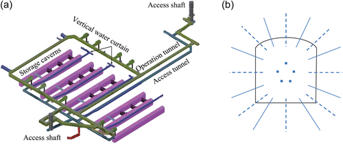
The JRC project consists primarily of two vertical access shafts, five storage caverns, two levels of operation and access tunnels, and a vertical water curtain system (Figure 1a). The access shafts, located on Jurong Island, extend down to a depth of 150 m. The storage caverns, with a storage capacity of 1.5 million m3, are constructed beneath the Banyan Basin, positioned between the two access shafts. The access tunnels are situated above the storage caverns to enhance hydraulic containment and ensure the secure confinement of stored oil within the caverns. The operation tunnels are located above the access tunnels to supply the vertical water curtain system, which segregates different storage materials across these caverns.
This study focused on the grouting operation during the excavation of an operation tunnel with a length of about 200 m. The sedimentary rocks, such as sandstone, siltstone, and mudstone, are heavily folded and faulted with discontinuous aligning either parallel with or perpendicular to the fold strike (Zhao et al., 1999). These rock materials are of good quality, with an average uniaxial compressive strength of around 100 MPa. The rock masses are intersected by several joint sets, which serve as major passages for water inflow. Before advancing each round of drill and blast, 15-m-long probe holes with a diameter of 54 mm were drilled to measure the water inflow rate from the excavation face. If the inflow rate exceeded a certain threshold, grouting holes were drilled on a grouting screen and injected with a pressured water–cement mixture. After that, control holes were drilled to assess the effectiveness of the grouting operation.
The grouting holes were classified into three rounds on each grouting screen (Figure 1b). The first-round holes were uniformly distributed around the tunnel periphery. The second-round holes were drilled midway between the neighboring first-round holes. The third-round holes were scattered and determined by onsite engineers to reinforce regional grouting efficiency. The grouting holes from two neighboring grouting screens had an overlapping distance of 5 m to ensure the effective sealing of cross-sectional passages for water inflow.
The rock mass parameters, hydrogeological data, and grouting data were collected to establish the machine learning models. The rock mass parameters included the rock quality designation (RQD), the Q value, and rock mass rating (RMR), which were obtained from the excavation face mapping and borehole logs. The hydrogeological data consisted of the water flow rate and water pressure. The grouting data contained the water–cement ratio, grouting pressure, and grout volume.
2.2 Data analysis
Figure 2 presents the data analysis flowchart, which consists of four steps: data collection, data processing, model selection, and model deployment. In the first step, the raw data include the rock mass parameters, hydrogeological properties, and grouting data. The second step involves data pre-processing and feature engineering. During data pre-processing, data cleaning, such as addressing anomalies related to grout choking and machine malfunctions, was conducted, followed by data normalization to minimize the impact of varying input magnitudes. For feature engineering, the principal component analysis was carried out using the scikit-learn package for Python (Pedregosa et al., 2011) to identify the correlations and variances among these inputs (Jolliffe, 2002). The objective of principal component analysis is to determine the direction of the principal component (PC), where the projected data show the maximum variance. The underlying principle involves projecting the original inputs, defined by their initial coordinates (e.g., x1, x2, x3, etc.), into a rotated space with new coordinates (e.g., PC1, PC2, PC3, etc.), where each PC is a linear combination of the original inputs. The processed data were then split into two data sets: the training and testing data sets. The training data set trained the machine learning model, enabling the model to learn and fit the data, while the testing data set evaluated the generalization capabilities of the model and helped prevent overfitting. Finally, both the data sets were used to assess the performance of the model.

ANN and DT were selected to study the spatial dependence of grouting efficiency, as both the methods are well suited for solving regression problems. The ANN model is highly effective at capturing complex, nonlinear relationships within the data, making it particularly suitable for modeling spatial patterns and interactions. Meanwhile, the DT model offers a straightforward and intuitive approach, providing a clear, step-by-step structure that makes it easy to identify key decision rules.
The ANN model is advantageous for approximating nonlinear relationships between inputs and outputs (Hornik et al., 1989). A typical ANN structure consists of an input layer with a number of neurons equal to the number of inputs, one or more hidden layers, and an output layer with neurons corresponding to the number of outputs. Each neuron computes a weighted sum of the outputs from the previous layer, plus a bias term. This sum is then passed through an activation function to produce the neuron's output. Activation functions introduce the nonlinearity that enables the ANN model to approximate complex relationships. The performance of the ANN model is evaluated using the mean squared error (MSE) between the predicted and measured values, which serves as the cost function. This cost function is minimized using backpropagation algorithms, such as the Levenberg–Marquardt backpropagation algorithm, to adjust the weights and biases throughout the network.
The DT model has a tree-like structure that is effective for both classification and regression tasks, as well as for modeling decisions and their possible outcomes. In this structure, each internal node represents a decision based on a specific feature, each branch represents the outcome of that decision, and each leaf node represents the outcome. After recursively splitting the data set into small subsets based on the value of a chosen feature, the DT model selects the feature that best separates the data according to a specific criterion, such as Gini Impurity or Information Gain for classification tasks, or MSE for regression tasks, to minimize impurity or variance within each subset. Once the optimal feature is selected, the data set is divided into subsets based on the value of this feature. This process of selecting the best feature and splitting the data is repeated recursively for each subset, continuing until a stopping criterion is met, such as reaching a maximum tree depth, having a minimum number of samples per node, or finding that further splitting does not significantly reduce impurity.
2.3 Input selection
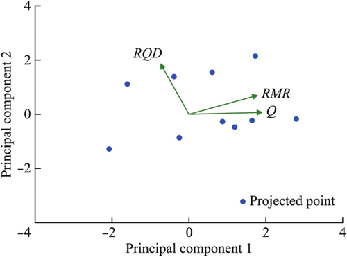
The principal component analysis was performed on RQD, Q, and RMR. Upon decomposing the principal components, PC1 was identified as a linear combination of the rock mass parameters: PC1 = −0.27 × RQD + 0.7 × Q + 0.66 × RMR. The absolute values of the coefficients in this equation indicate the contributions of original inputs to the principal component. In this case, PC1 is most strongly influenced by Q and RMR. Figure 3 illustrates the projection of RQD, Q, and RMR onto the two-dimensional space defined by PC1 and PC2. Since PC1 captures the majority of the variance from the combined RQD, Q, and RMR, it serves as a reliable indicator of rock mass quality. The other inputs include the water flow rate, water pressure, grouting pressure, and the coordinates of grouting holes on the excavation face, which together describe the hydrogeological and grouting information. Therefore, the supervised machine learning models use six inputs to predict the output, that is, grout volume.
3 RESULTS
The correlation coefficients obtained from the ANN and DT models are compared in Table 1. Although the DT model, with a maximum tree depth as 10 and a minimum sample number per node as 5, performs best on the training data set, it shows signs of overfitting, as its performance on the testing data set is poor. The ANN model provides more balanced regression results across both the training and testing data sets. Therefore, the ANN model is selected and refined to predict the grout volume.
| Model | Structure | R (training) | R (testing) | R (overall) |
|---|---|---|---|---|
| ANN | Hidden neuron: 10 | 0.878 | 0.491 | 0.801 |
| DT | Maximum tree depth: 10 Minimum sample number: 5 |
0.930 | 0.390 | 0.822 |
Maximum tree depth: 5 Minimum sample number: 5 |
0.793 | 0.435 | 0.721 | |
Maximum tree depth: 3 Minimum sample number: 10 |
0.732 | 0.551 | 0.696 |
To enhance the ANN model and improve the prediction of grout volume, its hyperparameters are carefully tuned through the following steps. First, the data are split into three data sets, that is, the training data set (70%) to adjust the network weights and biases, the validation set (15%) to fine-tune the hyperparameters and prevent overfitting by determining when to stop training, and the testing data set (15%) to estimate the model performance on unseen data. Several hidden layer configurations with different numbers of neurons (e.g., 30, 40, 50, and 60) were tested, and the best-performing ANN structure has one hidden layer with 40 neurons (Table 2).
| Number of neurons | R (training) | R (validation) | R (testing) | R (overall) |
|---|---|---|---|---|
| 30 | 0.783 | 0.536 | 0.505 | 0.724 |
| 40 | 0.773 | 0.747 | 0.661 | 0.748 |
| 50 | 0.655 | 0.547 | 0.309 | 0.572 |
| 60 | 0.772 | 0.354 | 0.574 | 0.671 |
| R (training) | R (validation) | R (testing) | R (overall) | ||
|---|---|---|---|---|---|
| Training algorithm | Levenberg–Marquardt | 0.773 | 0.746 | 0.661 | 0.748 |
| Bayesian regularization | 0.704 | 0.496 | – | 0.670 | |
| Scaled conjugate gradient | 0.749 | 0.457 | 0.516 | 0.687 | |
| Activation function | Tangent sigmoid + pure linear | 0.773 | 0.746 | 0.661 | 0.748 |
| Log sigmoid + pure linear | 0.806 | 0.597 | 0.518 | 0.724 | |
| Rectified linear unit + pure linear | 0.793 | 0.447 | 0.622 | 0.723 | |
| Regularization coefficient | 0 | 0.773 | 0.746 | 0.661 | 0.748 |
| 0.1 | 0.801 | 0.722 | 0.719 | 0.763 | |
| 0.5 | 0.834 | 0.720 | 0.621 | 0.777 | |
| 0.9 | 0.624 | 0.774 | 0.680 | 0.657 |
The first term in Equation (2) represents the traditional MSE used in the cost function, while the second term introduces the L2 regularization. This regularization term helps prevent individual neuron weights from becoming too large, thereby reducing the risk of overfitting. The regularization coefficient is a non-negative hyperparameter that determines the strength of regularization. Table 3 also shows its impact on the correlation coefficient, showing that a regularization coefficient of 0.5 provides the best performance of the ANN model. The Levenberg–Marquardt backpropagation algorithm was selected based on these results and then applied in the subsequent cases.
4 DISCUSSION
4.1 Spatial dependence in grouting performance
The ANN model, trained by the complete data set of grouting activities during the construction of the operation tunnel, achieves a correlation coefficient of 0.777. While using the overall data set of the grouting operation is common practice in underground engineering, the prediction of grout volume remains challenging due to the anisotropic and heterogeneous characteristics of surrounding rock masses. To enhance the reliability of the model in predicting grout volume, the ANN model was refined by incorporating the spatial factors that likely influence the grouting performance, such as the number of grouting holes in four quadrants of tunneling faces, the sequence of grouting screens along the tunnel axis, and the order of grouting rounds on the tunneling faces.
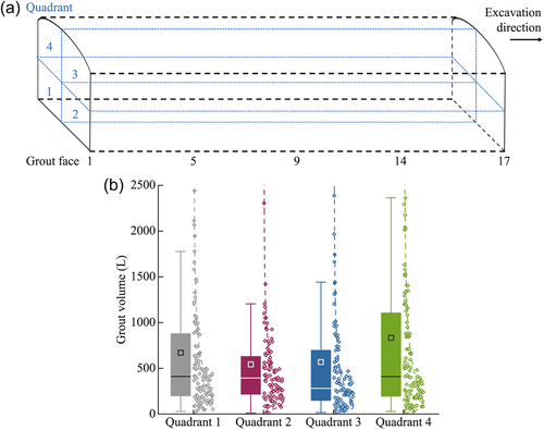
The tunneling face was first divided into four quadrants (Figure 4a). These quadrants contain different numbers of grouting points, such as 120 grouting points in Quadrant 1, 100 grouting points in Quadrant 2, 107 grouting points in Quadrant 3, and 128 grouting points in Quadrant 4. The corresponding average grout volumes are 670, 542, 568, and 833 L, respectively. The boxplots illustrate the uneven distribution of grout volume used in the four quadrants (Figure 4b). The correlation coefficients for the grout volume predicted by the refined model vary randomly in the four quadrants (Figure 5).
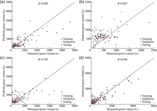
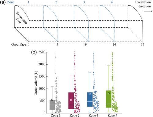
17 grout screens were then grouped into four zones along the tunnel axis, such as Zone 1 with grouting screens 1–4, Zone 2 with grouting screens 5–8, Zone 3 with grouting screens 9–13, and Zone 4 with grouting screens 14–17 (Figure 6a). The boxplot and the distribution curve also show different amounts of grout volume used in the four zones (Figure 6b). The correlation coefficients for the grout volume predicted by the ANN model remain fluctuated compared to the correlation coefficient obtained from the ANN model trained by the overall data (Figure 7).
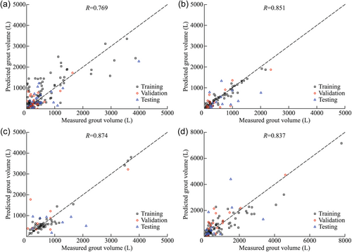
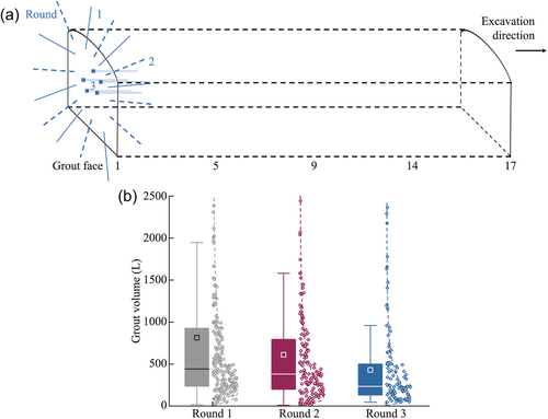
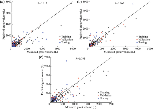
The grouting data were finally grouped following the order of grouting rounds on the tunneling faces (Figure 8a). Each grout screen contained three grouting rounds. The grouting data from 17 grout screens were divided into three groups and then used to re-train and fine-tune the ANN model for each specific round. The grouped data are represented in the boxplots, where the top edge, the middle line, and the bottom edge denote 75%, 50%, and 25% percentile values of grout volume, respectively, and the scatter plots are overlaid with the best-fit lognormal distribution curves (Figure 8b). This figure illustrates that the grout volume reduces with subsequent grouting rounds, indicating the effectiveness of grouting activities. The refined model predicts the grout volume with correlation coefficients of 0.813, 0.862, and 0.793 for the three rounds (Figure 9), which demonstrate that the performance of the model improves when using the grouped data based on the order of grouting rounds, in comparison to using the overall data set. The results indicate that the training strategy is reasonable by following the measured grouting operation during tunnel construction.
4.2 Validation
After comparing with the three spatial scenarios, we found that incorporating the order of grouting rounds on the tunneling faces as a training strategy improves the prediction accuracy compared to considering the number of grouting holes in four quadrants of tunneling faces and the sequence of grouting screens along the tunnel axis. To validate this finding, the rock mass parameters, hydrogeological data, and grouting records were collected from the excavation of the second operation tunnel, which is approximately 190 m long and includes 25 grout screens from the same project. The data set consists of 674 grouting records, including 316, 181, and 177 for Round 1, Round 2, and Round 3, respectively. When trained on the complete data set, the ANN model shows a correlation coefficient of 0.706. We then followed the three spatial scenarios (Figures 4, 6, and 8a) and refined the ANN model by incorporating the spatial factors, such as the number of grouting holes in four quadrants of tunneling faces, the sequence of four grouting screens along the tunnel axis, and the order of three grouting rounds on the tunneling faces. The correlation coefficients for three spatial scenarios are higher than 0.706, indicating that three spatial scenarios can improve the performance of the ANN model (Table 4). Notably, the training strategy considering the order of grouting rounds achieves the highest average correlation coefficient, consistent with the results obtained from the first tunnel.
| Spatial scenario | R | Average R | |||
|---|---|---|---|---|---|
| Four quadrants of tunneling faces | Quadrant 1 0.781 |
Quadrant 2 0.700 |
Quadrant 3 0.767 |
Quadrant 4 0.772 |
0.755 |
| Four zones along tunnel axis | Zone 1 0.784 |
Zone 2 0.742 |
Zone 3 0.796 |
Zone 4 0.827 |
0.787 |
| Three rounds on tunneling faces | Round 1 0.767 |
Round 2 0.771 |
Round 3 0.853 |
- | 0.797 |
This study emphasizes the importance of integrating physical significance into the training of machine learning models to enhance prediction accuracy. However, identifying these physical insights among numerous physical and mechanical factors in engineering practice remains a challenge. This raises a critical question: how can we effectively extract and incorporate essential physical parameters into model training? One potential solution is the use of advanced algorithms, such as the dual-stage attention-based recurrent neural network, which can help identify dominant factors and their evolution during the grouting process (Fang & Wu, 2024). This neural network, which incorporates an attention mechanism, excels in discerning the relative importance of multiple controlling factors (Qin et al., 2017). Factors that have a significant impact on prediction accuracy should be prioritized in model training to better reflect physical significance and improve predictive performance.
5 CONCLUSIONS
This paper focuses on predicting grout volume to address excess water inflow in tunnel excavation. An ANN model was developed using the data set from a tunnel project and enhanced through feature engineering, model selection, hyperparameter tuning, and regularization. The results demonstrate that the ANN model performs better than the DT model. The refined ANN model is further used to examine the spatial dependence of grouting efficiency. A comparison of predicted and measured grout volumes across different spatial scenarios highlights that the training strategy can be improved by integrating the grouting process. This method enables site engineers to analyze grouting data from both spatial and grouting sequence perspectives for efficient control of excess water inflow. The finding should be further validated in other underground projects before being applied to assist onsite engineers in real-world applications. This is because the finding may be case-dependent, as grouting data can vary based on geological conditions. Additionally, other big data technologies could enhance the prediction of grout volume. For instance, using digital twins can help visualize the grouting progress more efficiently, and applying deep learning applied to larger data sets may further improve the model performance. Particularly, transfer learning utilizes grouting knowledge gained from one tunnel to enhance grouting performance in new settings, resulting in more reliable predictions across different cases affected by various geological conditions.
ACKNOWLEDGMENTS
This study was supported by the Ministry of Education of Singapore, under Academic Research Fund Tier 1 (Grant Number RG143/23). The authors would like to express their sincere gratitude to the late Professor Zhiye Zhao in Nanyang Technological University, Singapore. He initiated this study and guided the early stage of the research.
CONFLICT OF INTEREST STATEMENT
The authors declare no conflict of interest.
Biography

Wei Wu is an associate professor at Nanyang Technological University (NTU), Singapore. He received his PhD degree at the Swiss Federal Institute of Technology in Lausanne (EPFL), Switzerland. Prior to joining NTU, he was a postdoctoral scholar at Stanford University. He currently serves as the President of Society for Rock Mechanics & Engineering Geology (Singapore) and the Associate Editor for International Journal of Rock Mechanics and Mining Sciences. His research focuses on experimental geophysics and energy geomechanics, with focus on underground space development, geo-energy extraction and storage, urban geophysics, and induced geohazards due to climate change and energy extraction.
Open Research
DATA AVAILABILITY STATEMENT
The data that support the findings of this study are available on request from the corresponding author. The data are not publicly available due to privacy or ethical restrictions.


