An Efficient Deep Learning Framework for Automated Epileptic Seizure Detection: Toward Scalable and Clinically Applicable Solutions
Funding: This research was supported by the National Natural Science Foundation of China (No. 62271291), the Key Program of the Natural Science Foundation of Shandong Province (No. ZR2020LZH009), and the Shenzhen Science and Technology Program (GJHZ20220913142607013).
ABSTRACT
In this study, we present an efficient epileptic seizure detection framework driven by a graph convolutional neural network (GCNN). Unlike conventional methods that primarily rely on local features or complex feature engineering, our GCNN-based approach explicitly encodes the spatial dependencies among electroencephalogram (EEG) electrodes, thereby capturing more comprehensive spatiotemporal features. A minimal preprocessing pipeline, consisting only of bandpass filtering and segmenting, reduces system complexity and computational overhead. On the CHB-MIT scalp EEG database, our method achieved an average accuracy of 98.64%, sensitivity of 99.49%, and specificity of 98.64% at the segment-based level and sensitivity of 96.81% with FDR of 0.27/h at the event-based level. On the SH-SDU database we collected, the method yielded segment-based accuracy of 95.23%, sensitivity of 92.42%, and specificity of 95.25%, along with event-based sensitivity of 94.11%. The average testing time for 1 h of multi-channel EEG signals is 3.89 s. These excellent results and low-computation design make the framework especially suited for clinical applications, advancing EEG-based epilepsy diagnostics and improving patient outcomes.
1 Introduction
Epilepsy is a prevalent chronic neurological disorder that affects individuals of all ages (Andersson et al. 2024; Beghi 2020; Cai et al. 2023). According to the World Health Organization (WHO), approximately 50 million people around the world suffer from epilepsy. Epileptic seizures are usually caused by the suddenly abnormal discharges, or excessively synchronous activity of neurons in the brain, resulting in temporary brain dysfunction, along with neurobiological, cognitive, psychological, and social consequences (Fisher et al. 2005; Sebe and Baraban 2011). Timely and accurate diagnosis of epilepsy is essential to initiate antiepileptic treatments, reduce seizure frequency, and mitigate associated complications.(Kadam 2018; Moshé et al. 2015). Electroencephalogram (EEG) is the electrical signal generated by neurons in the brain and can be recorded with multiple electrodes placed on the scalp (Casson et al. 2010). EEG is the most effective method to study human brain activity, especially for the diagnosis of epilepsy-related diseases (Faust et al. 2015; Rafiei et al. 2024; Wong et al. 2023). For long-term EEG monitoring, neurologists may need to manually review hours or days of EEG recordings based on experience, which is time-consuming and not cost-effective. Therefore, there is an urgent demand for automatic seizure detection systems with higher accuracy and lower false detection rate (FDR) to assist physicians in analyzing EEG data more efficiently (G. Y. Liu et al. 2020).
Since Gotman first proposed the method of automatic identification of epileptic seizures based on EEG in 1982, the research of seizure detection has developed rapidly (Gotman 1982). Early seizure detection methods are mainly based on hand-crafting EEG features and traditional machine learning methods, among which commonly used classification models include support vector machine (SVM; Bajaj and Pachori 2012; Kaleem et al. 2021; Nandan et al. 2010; Nicolaou and Georgiou 2012), random forest (Donos et al. 2015; Mursalin et al. 2017), Bayes linear discriminant analysis (BLDA; Zhou et al. 2013), Naïve Bayes (NB; Amin et al. 2015; Selvakumari et al. 2019), and artificial neural networks (ANNs; Alkan et al. 2005; Guo et al. 2010; Webber et al. 1996). At the same time, machine learning techniques have been widely used in fields such as cancer detection and prediction, achieving better results (Mostafa et al. 2024). The advantage of conventional machine learning models lies in their limited complexity and high interpretability. However, it is a challenging task to extract complex features from EEG data using feature engineering, and the process of feature extraction is usually time-consuming, which affects the efficiency of seizure detection in practical scenarios (Shoeibi et al. 2021).
In recent years, with the rapid development of deep learning technology, it has been used in assisted diagnosis of diseases (Hassan et al. 2024). Meanwhile, such deep neural networks have also been widely applied in the field of seizure detection (Cui et al. 2024; H. T. Li et al. 2024; Omar and Abd El-Hafeez 2024). Those models can achieve high-precision classification and prediction by learning features and patterns in EEG data. The most commonly used deep learning model for seizure detection is the convolutional neural network (CNN; Daoud and Bayoumi 2019; Huang et al. 2022; C. Y. Li et al. 2025, 2023; D. S. Liu et al. 2023) and long short-term memory networks (LSTMs; Hu et al. 2020; Y. Li et al. 2020). Compared with traditional machine learning algorithms, CNN and LSTM have the ability to automatically extract features and act as an end-to-end classifier. It should be noted that CNN was originally proposed to solve the problem of image recognition, while LSTM is more adept at handling natural language processing, and their advantage lies in processing Euclidean data such as images and speech. CNN can usually capture local features of EEG, and LSTM can utilize the temporal correlation information of EEG without considering their global and spatial connectivity. Since electrodes for EEG recording have positional relationships, it is necessary to consider the spatial connectivity between electrodes for better capturing spatial features of multi-channel EEG (Song et al. 2020).
The deep learning techniques related to graph data processing are also rapidly iterating, and a variety of related techniques are widely used in the intelligent detection and prediction of various diseases (Eliwa et al. 2023, 2024). Graph CNN (GCNN) was proposed to process non-Euclidean spatial data and could capture global and local features (Asif et al. 2021). Unlike traditional CNNs, GCNNs can capture both local and global features of EEG by modeling electrodes as nodes in a graph, where their connections reflect spatial proximity or functional similarity. By performing convolution operations on the graph structure, it can capture the relationships between graph nodes and obtains a more accurate representation for spatial data. Different from the traditional CNN, GCNN requires an adjacency matrix to define the relationship between nodes based on the graph structure. Therefore, reasonable construction of an adjacency matrix is a crucial step to improve the performance of GCNN. In seizure detection tasks, the electrodes for EEG signal acquisition have spatial relationships, which can be represented as a graph structure, with each electrode as a node in the graph. The connection relationship can be defined by indicators such as the distance between adjacent electrodes and their functional similarity. Despite these advantages, most seizure detection methods have been validated on a single EEG database, raising concerns about their generalizability to diverse patient populations (Raghu et al. 2020).
In this work, we propose a GCNN-based seizure detection framework that addresses these challenges. The system incorporates a simplified preprocessing pipeline and focuses on cross-database validation using the CHB-MIT pediatric database and the SH-SDU database, which includes middle-aged and elderly patients. This approach ensures robust performance across varied populations, demonstrating the potential for clinical deployment. By achieving high accuracy and low FDR with minimal computational requirements, our method lays the foundation for a practical, scalable solution to improve epilepsy diagnosis and patient care.
2 Database
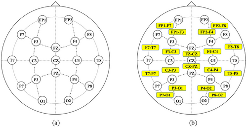
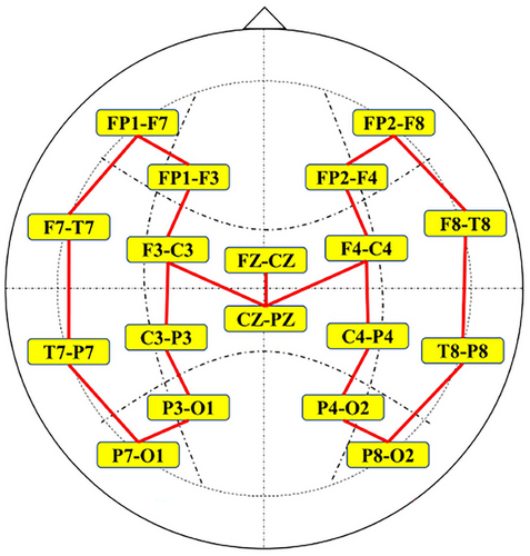
The publicly available CHB-MIT Scalp EEG database contains EEG recordings from 23 pediatric subjects with intractable seizures (Shoeb 2009). There is a total of 24 case recordings in the database, all of which were obtained using electrode positions according to the international 10–20 system with a signal sampling rate of 256 Hz. In this experiment, EEG recordings with a total duration of 979 h and 184 seizure events from the CHB-MIT database were used to evaluate the seizure detection method. The summary of seizure events from the 24 cases in the CHB-MIT database is presented in Table 1. Most EEG recordings contain 23 bipolar channels (24 or 26 in a few cases), and 18 common bipolar channels in 24 cases were selected for uniformity, which are FP1-F7, F7-T7, T7-P7, P7-O1, FP1-F3, F3-C3, C3-P3, P3-O1, FP2-F4, F4-C4, C4-P4, P4-O2, FP2-F8, F8-T8, T8-P8, P8-O2, FZ-CZ, and CZ-PZ. The specific electrode locations are illustrated in Figure 1.
| Case | Sex | Age | Number of seizure events | Number of seizure events for training | Total seizure duration (min) | Total electroencephalogram (EEG) duration (h) |
|---|---|---|---|---|---|---|
| CHB01 | F | 11 | 7 | 1 | 7.37 | 40.55 |
| CHB02 | M | 11 | 3 | 1 | 2.87 | 35.27 |
| CHB03 | F | 14 | 7 | 1 | 6.70 | 38.00 |
| CHB04 | M | 22 | 4 | 2 | 6.30 | 156.07 |
| CHB05 | F | 7 | 5 | 1 | 9.30 | 39.00 |
| CHB06 | F | 1.5 | 10 | 5 | 2.55 | 66.74 |
| CHB07 | F | 14.5 | 3 | 1 | 5.42 | 67.05 |
| CHB08 | M | 3.5 | 5 | 1 | 15.32 | 20.01 |
| CHB09 | F | 10 | 4 | 1 | 4.60 | 67.87 |
| CHB10 | M | 3 | 6 | 1 | 6.55 | 50.02 |
| CHB11 | F | 12 | 3 | 1 | 13.43 | 34.79 |
| CHB12 | F | 2 | 27 | 8 | 16.48 | 20.69 |
| CHB13 | F | 3 | 12 | 3 | 8.92 | 33.00 |
| CHB14 | F | 9 | 8 | 4 | 2.82 | 26.00 |
| CHB15 | M | 16 | 20 | 2 | 33.20 | 40.01 |
| CHB16 | F | 7 | 10 | 5 | 1.40 | 19.00 |
| CHB17 | F | 12 | 3 | 1 | 4.88 | 21.01 |
| CHB18 | F | 18 | 6 | 2 | 5.28 | 35.63 |
| CHB19 | F | 19 | 3 | 1 | 3.93 | 29.93 |
| CHB20 | F | 6 | 8 | 2 | 4.90 | 27.60 |
| CHB21 | F | 13 | 4 | 2 | 3.32 | 32.83 |
| CHB22 | F | 9 | 3 | 1 | 3.40 | 31.00 |
| CHB23 | F | 6 | 7 | 3 | 7.07 | 26.56 |
| CHB24 | N/A | N/A | 16 | 1 | 8.52 | 21.30 |
| Summary | — | 9.98 | 184 | 51 | 184.53 | 979.93 |
It is noted that the CHB-MIT database consists of EEG data from pediatric epilepsy patients, with an average age of 10 years for the cases. In order to include patients from a wider age range, we collected EEG data from 8 epilepsy patients in the Second Hospital of Shandong University (SH-SDU) in Jinan, China. These patients had an average age of 46 years. The SH-SDU database included 73.64 h of EEG signals with a sampling rate of 500 Hz and a total of 86 seizure events. We selected 18 unipolar channels, namely, FP1, FP2, F3, F4, C3, C4, P3, P4, O1, O2, F7, F8, T3, T4, T5, T6, FZ, and PZ, which were in similar positions to the bipolar locations in the CHB-MIT database. The information for the SH-SDU database is shown in Table 2.
| Case | Sex | Age | Number of seizure events | Number of seizure events for training | Total seizure duration (min) | Total EEG duration (h) |
|---|---|---|---|---|---|---|
| 01 | F | 28 | 16 | 6 | 9.83 | 17.08 |
| 02 | M | 61 | 10 | 1 | 36.80 | 16.04 |
| 03 | M | 34 | 10 | 2 | 8.70 | 12.00 |
| 04 | M | 79 | 23 | 4 | 17.05 | 6.00 |
| 05 | M | 45 | 3 | 1 | 2.97 | 6.00 |
| 06 | F | 37 | 6 | 2 | 2.30 | 3.77 |
| 07 | F | 38 | 3 | 1 | 1.73 | 6.00 |
| 08 | M | 49 | 15 | 2 | 27.35 | 12.00 |
| Summary | — | 46.38 | 86 | 20 | 106.73 | 73.64 |
3 Methods
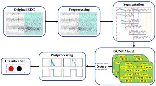
To explore the relationship between different electrodes and extract hidden feature information, GCNN is deployed to identify seizure events in multi-channel scalp EEG. The method is mainly composited of four parts: preprocessing, segmentation, GCNN model, and postprocessing. The overall flowchart of the method is shown in Figure 2. Except for down-sampling the 500 Hz EEG signal of the SH-SDU database to 256 Hz in the preprocessing stage, the rest of the process is consistent with the CHB-MIT database.
3.1 Preprocessing and Segmentation
To highlight the superiority of the GCNN model, this work aims to simplify the preprocessing process and avoid time-consuming feature extraction used in most seizure detection methods. We only deploy a filter with a frequency range of 0.1–48 Hz on raw EEG signals to reserve seizure features and remove artifacts and power-line noise (Cui et al. 2024; Dash et al. 2020). The comparison before and after filtering is shown in Figure 3. As the length of ictal data is significantly less than that of interictal data, this results in an imbalance of seizure and non-seizure data in the training set, which will seriously affect the model's detection accuracy. Consequently, data imbalance is a prevalent challenge in seizure detection. To address this issue, we employed a data augmentation technique to increase the amount of seizure segments (Cui et al. 2024). For this reason, we split the ictal data into 1-s segments and perform 75% overlapping data augmentation as shown in Figure 4. Meanwhile, we select interictal data that are four times the duration of the ictal data and divide them into 1-s segments without overlapping. For the testing set, all EEG recordings are sliced into 1-s segments.

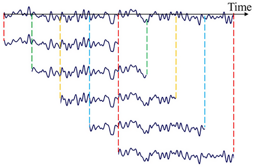
Table 3 presents the detailed data information about two databases used for training and testing. For the CHB-MIT database, after augmentation, there were 10,350 seizure segments and 10,350 non-seizure segments (2.30 h before augmentation) used for training. The number of segments used for testing was 3,519,468 (977.63 h in total). For the SH-SDU database, after augmentation, there were 7260 seizure segments and 7260 non-seizure segments (1.61 h before augmentation) for training. The number of segments for testing was 259,308 (72.03 h in total).
| Database | Total duration | Seizure events | Training events | Training segments | Testing events | Testing segments |
|---|---|---|---|---|---|---|
| CHB-MIT | 979.93 h | 184 | 51 | 20,700 | 133 | 3,519,468 |
| SH-SDU | 73.64 h | 86 | 20 | 14,520 | 66 | 259,308 |
3.2 Graph Convolutional Model
Compared with the traditional CNN models, GCNN is adept at dealing with the topological structure of a graph. The multi-channel EEG signals could be represented as a topological graph. The GCNN model can perform adaptive feature extraction on the topological structure data, so as to capture the topological features in the multi-channel EEG signals and improve the performance of seizure detection. A key aspect of implementing GCNN for seizure detection is to correctly define the adjacency matrix that characterizes the relationships of various vertex nodes to set up the relationships between the 18 bipolar channels. With the accumulation of experiments, the optimal connection relationship between the 18 channels is ultimately obtained as shown in Figure 5.
Algorithm 1 Graph convolutional model.
| Input: Preprocessed EEG segments {X}, adjacency matrix A |
| Output: Seizure prediction labels {} |
| 1: For each 1-s EEG segment : |
| 2: Construct graph Gi = (Vi, Ei) with 18 nodes and edges from A |
| 3: Assign node features Fi from segment xi |
| 4: Assign label |
| 5: Initialize GCNN model with 4 GraphConv layers and 2 FC layers |
| 6: for epoch = 1 to N do |
| 7: for each training batch B do |
| 8: Forward propagate through GCNN |
| 9: Compute cross-entropy loss L |
| 10: Backpropagate and update parameters using Adam optimizer |
| 11: Load best model weights |
| 12: for each test batch B′ do |
| 13: Perform inference to get seizure scores si |
| 14: Apply moving average smoothing on {si} |
| 15: Threshold scores to get binary outputs |
| 16: Apply collaring to refine seizure boundaries |
| 17: Evaluate results against expert labels: |
| Compute accuracy, sensitivity, specificity, F1 score, AUC, FDR |
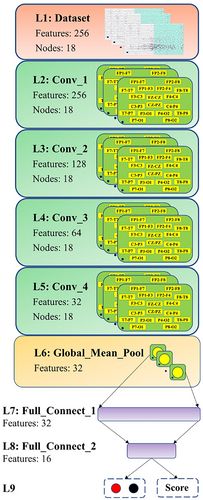
As presented in Table 4 and Figure 6, the designed GCNN model consists of four graph convolutional layers, one global mean pooling layer, and two fully connected layers. The preprocessed EEG data are organized into a data format of 18 nodes × 256 features and inputted into the graph convolutional layers. Those EEG data first pass through four graph convolutional layers, where the number of nodes remains the same, while the number of features is sequentially reduced to 256, 128, 64, and 32. After four convolutional layers, the data format of the output becomes 18 nodes × 32 features. To further integrate the features, the output is sent to the global mean pooling layer, where the feature vectors of each node are averaged. Finally, the model yields the EEG classification results through two fully connected layers with neurons of 16 and 2.
| Layer no. | Layer type | Input shape | Output shape | Parameters count | Description |
|---|---|---|---|---|---|
| 1 | GraphConv (conv1) | (18 nodes, 256 features) | (18 nodes, 128 features) | 32,896 | Graph convolution + ReLU + Dropout (p = 0.3) |
| 2 | GraphConv (conv2) | (18 nodes, 128 features) |
(18 nodes, 64 features) |
8256 | Graph convolution + ReLU + Dropout (p = 0.3) |
| 3 | GraphConv (conv3) |
(18 nodes, 64 features) |
(18 nodes, 32 features) |
2080 | Graph convolution + ReLU + Dropout (p = 0.3) |
| 4 | GraphConv (conv4) |
(18 nodes, 32 features) |
(18 nodes, 32 features) |
1056 | Graph convolution + ReLU + Dropout (p = 0.3) |
| 5 | GlobalMeanPooling |
(18 nodes, 32 features) |
(1 × 32 vector per sample) | — | Averages over 18 graph nodes |
| 6 | Linear (fc1) | (1 × 32) | (1 × 16) | 528 | Fully connected + Dropout (p = 0.5) |
| 7 | Linear (fc2) | (1 × 16) | (1 × 2) | 34 | Output layer for 2-class classification |
| Total | — | — | 44,850 |
In this work, ReLu is selected as the activation function of the model, which can effectively solve the problem of gradient vanishing. To avoid overfitting, a dropout layer is added after each graph convolutional layer to randomly drop out a certain percentage of neurons to make the model more robust. The dropout rate is set to 0.3. To solve the binary classification problem in seizure detection, the cross-entropy is chosen as the loss function. In the model training process, the Adam optimization algorithm is used, which has the characteristic of adaptive matrices and can accelerate the convergence of the model. The learning rate is set to 0.001 for all cases, the maximum number of epochs to 200, and the mini-batch size to 64. The hyperparameters used by the model during training and testing are listed in Table 5.
| Parameter | Value |
|---|---|
| Learning rate | 0.001 |
| Batch size | 64 |
| Epochs | 200 |
| Dropout rate | 0.3 |
| Optimizer | Adam |
| Loss function | Cross-entropy |
3.3 Postprocessing
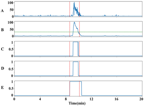
Smoothed scores are compared with a fixed threshold (Thr) to obtain a binarized result, with scores greater than Thr of 1 representing a seizure segment and scores less than Thr of 0 representing a non-seizure segment. Although score smoothing is effectively able to eliminate false positives, it may cause a decrease in the accuracy of detection results. To compensate for this deficiency, the collar technique is applied to extend K points at the beginning and end of a segment labeled as a seizure event (Temko et al. 2011). In order to reduce the number of incorrect labels, seizures recognized by the detection method are considered a single seizure event if they are less than 180 s apart from each other. The three postprocessing parameters N, Thr, and K are adjusted for each case to obtain the optimal results. Figure 7 illustrates the general process of postprocessing.
4 Results
All experiments were carried out in Matlab 2022a and PyTorch environment (Python 3.6) running on an Intel(R) Core (TM) i9-9820X CPU and a 32 GB NVIDIA GeForce RTX 2080 SUPER GPU. During the testing phase, segment-based and event-based evaluation criteria were used to evaluate the seizure detection performance of the proposed method. Under the given hardware conditions, the proposed model required an average training time of 65.38 s when trained using the hyperparameters specified in Tables 4 and 5. Additionally, the average time to process 1 h of multichannel EEG signals during testing was 3.89 s. These results demonstrate the lightweight feature of the proposed model and its real-time potential in automatic seizure detection.
The results of the segment-based assessment on the CHB-MIT database are provided in Table 6. The average accuracy was 99.49%, and the average sensitivity and specificity were both 98.64%; for the F1 score, the proposed model got 98.65%, and 98.62% of AUC at the same time. In 21 cases, the sensitivity reached 100%. Over 99% accuracy and specificity were achieved in more than half of the cases so as the F1 score and the AUC metrics. However, the accuracy in the cases CHB06 and CHB16 was lower at 96%, possibly due to the shorter duration of seizure events in these cases, that is, the average duration was 15.3 and 8.4 s, respectively. The segment-based evaluation on the SH-SDU database is presented in Table 7. The results were yielded with a mean accuracy, sensitivity, and specificity of 92.42%, 95.23%, and 95.25%, respectively. At the same time, a mean F1 score of 94.80% and AUC of 95.04% were recorded.
| Case | Sensitivity (%) | Accuracy (%) | Specificity (%) | F1 score (%) | Area under the curve (AUC; %) |
|---|---|---|---|---|---|
| CHB01 | 100 | 99.87 | 99.87 | 99.78 | 99.73 |
| CHB02 | 100 | 99.76 | 99.76 | 99.69 | 99.64 |
| CHB03 | 100 | 97.58 | 97.57 | 97.61 | 97.58 |
| CHB04 | 100 | 98.56 | 98.56 | 98.45 | 98.56 |
| CHB05 | 100 | 99.86 | 99.86 | 99.78 | 99.81 |
| CHB06 | 100 | 96.34 | 96.34 | 96.41 | 96.52 |
| CHB07 | 100 | 99.76 | 99.76 | 99.79 | 99.75 |
| CHB08 | 100 | 99.42 | 99.41 | 99.38 | 99.29 |
| CHB09 | 100 | 99.77 | 99.77 | 99.68 | 99.58 |
| CHB10 | 100 | 99.88 | 99.88 | 99.89 | 99.76 |
| CHB11 | 100 | 99.63 | 99.62 | 99.71 | 99.65 |
| CHB12 | 95.34 | 97.07 | 97.06 | 97.21 | 97.17 |
| CHB13 | 100 | 98.05 | 98.04 | 98.15 | 98.21 |
| CHB14 | 100 | 97.52 | 97.51 | 97.50 | 97.64 |
| CHB15 | 96.25 | 97.22 | 97.21 | 97.24 | 97.21 |
| CHB16 | 100 | 96.16 | 96.16 | 96.36 | 96.27 |
| CHB17 | 100 | 99.28 | 99.27 | 99.21 | 99.14 |
| CHB18 | 100 | 99.71 | 99.71 | 99.59 | 99.46 |
| CHB19 | 100 | 99.83 | 99.83 | 99.74 | 99.73 |
| CHB20 | 100 | 98.07 | 98.07 | 98.17 | 98.22 |
| CHB21 | 100 | 97.36 | 97.36 | 97.45 | 97.52 |
| CHB22 | 100 | 99.92 | 99.92 | 99.84 | 99.76 |
| CHB23 | 100 | 97.59 | 97.59 | 97.63 | 97.58 |
| CHB24 | 96.20 | 99.24 | 99.28 | 99.25 | 99.16 |
| Average | 99.49 | 98.64 | 98.64 | 98.65 | 98.62 |
| Case | Sensitivity (%) | Accuracy (%) | Specificity (%) | F1 score (%) | AUC (%) |
|---|---|---|---|---|---|
| 01 | 96.82 | 99.27 | 99.28 | 99.12 | 99.24 |
| 02 | 98.91 | 95.14 | 94.96 | 94.98 | 95.03 |
| 03 | 87.35 | 88.59 | 88.59 | 87.98 | 88.31 |
| 04 | 91.18 | 99.04 | 99.04 | 98.87 | 98.92 |
| 05 | 100 | 96.81 | 96.81 | 96.88 | 96.85 |
| 06 | 76.74 | 90.52 | 90.62 | 88.99 | 90.04 |
| 07 | 100 | 98.24 | 98.23 | 98.14 | 98.21 |
| 08 | 88.38 | 94.22 | 94.46 | 93.45 | 93.77 |
| Average | 92.42 | 95.23 | 95.25 | 94.80 | 95.04 |
To better investigate the performance of the proposed method in clinical practice, an event-based criterion assessment is also deployed. This involves two measures: event-based sensitivity, which is defined as the percentage of correctly detected seizure events in the total number of seizure events labeled by experts, and FDR, which represents the ratio of the number of false positives detected by the system to the total non-seizure time.
Based on the event-based evaluation, the method achieved the average sensitivity of 99.78% and the average FDR as 0.32/h on the CHB-MIT database as listed in Table 8. A total of 133 seizure events were tested, and 132 seizure events were correctly detected. Table 9 provides the event-based evaluation results of the method on the SH-SDU database. It indicates that out of the 67 tested seizure events, only 5 were not detected. The mean sensitivity was 90.82, and the mean FDR was 1.95/h.
| Case | Number of seizure events for testing | Number of seizure events detected | Sensitivity (%) | FPs | EEG duration for testing (h) | FDR (/h) |
|---|---|---|---|---|---|---|
| CHB01 | 6 | 6 | 100 | 0 | 40.4 | 0.00 |
| CHB02 | 2 | 2 | 100 | 7 | 35.17 | 0.20 |
| CHB03 | 6 | 6 | 100 | 8 | 37.9 | 0.21 |
| CHB04 | 2 | 2 | 100 | 76 | 155.87 | 0.49 |
| CHB05 | 4 | 4 | 100 | 0 | 38.85 | 0.00 |
| CHB06 | 5 | 5 | 100 | 43 | 66.64 | 0.65 |
| CHB07 | 2 | 2 | 100 | 2 | 66.95 | 0.03 |
| CHB08 | 4 | 4 | 100 | 0 | 19.76 | 0.00 |
| CHB09 | 3 | 3 | 100 | 2 | 67.77 | 0.03 |
| CHB10 | 5 | 5 | 100 | 1 | 49.92 | 0.02 |
| CHB11 | 2 | 2 | 100 | 1 | 34.74 | 0.03 |
| CHB12 | 19 | 18 | 94.74 | 18 | 20.39 | 0.88 |
| CHB13 | 9 | 9 | 100 | 12 | 32.75 | 0.37 |
| CHB14 | 4 | 4 | 100 | 40 | 25.85 | 1.55 |
| CHB15 | 18 | 18 | 100 | 16 | 39.56 | 0.40 |
| CHB16 | 5 | 5 | 100 | 9 | 18.95 | 0.47 |
| CHB17 | 2 | 2 | 100 | 4 | 20.91 | 0.19 |
| CHB18 | 4 | 4 | 100 | 3 | 35.53 | 0.08 |
| CHB19 | 2 | 2 | 100 | 1 | 29.83 | 0.03 |
| CHB20 | 6 | 6 | 100 | 17 | 27.5 | 0.62 |
| CHB21 | 2 | 2 | 100 | 14 | 32.73 | 0.43 |
| CHB22 | 2 | 2 | 100 | 0 | 30.9 | 0.00 |
| CHB23 | 4 | 4 | 100 | 23 | 26.36 | 0.87 |
| CHB24 | 15 | 15 | 100 | 5 | 21.2 | 0.24 |
| Average/Sum | 133 | 132 | 99.78 | 313 | 979.43 | 0.32 |
| Case | Number of seizure events for testing | Number of seizure events detected | Sensitivity (%) | FPs | EEG duration for testing (h) | FDR (/h) |
|---|---|---|---|---|---|---|
| 01 | 10 | 9 | 90 | 8 | 16.57 | 0.48 |
| 02 | 9 | 9 | 100 | 30 | 14.75 | 2.03 |
| 03 | 8 | 7 | 87.50 | 9 | 11.62 | 0.77 |
| 04 | 19 | 17 | 89.47 | 27 | 5.41 | 4.99 |
| 05 | 2 | 2 | 100 | 5 | 5.79 | 0.86 |
| 06 | 4 | 3 | 75 | 11 | 3.38 | 3.25 |
| 07 | 2 | 2 | 100 | 6 | 5.90 | 1.02 |
| 08 | 13 | 11 | 84.62 | 24 | 11.03 | 2.18 |
| Average/sum | 66 | 62 | 90.82 | 120 | 69.05 | 1.95 |
5 Discussion and Limitation
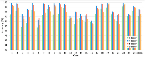
Generally, the overall performance and the complexity of the proposed model are associated with the number of layers in the GCNN. An excessive number of layers can lead to an increase in both the scale of model parameters and the computational cost, and may even cause overfitting. Meanwhile, too few layers will weaken the fitting ability and performance of the model. To investigate the impact of different numbers of GCNN layers on the model's classification performance, we conducted a series of controlled experiments by varying the number of GCNN layers while keeping all other parameters constant. The classification and detection results were then statistically analyzed. The classification results of the model in the cases of 3-, 4-, 5-, and 6-layer GCNNs are all shown in Figure 8. It is clear that 4-layer and 5-layer GCNNs outperform 3-layer and 6-layer GCNNs in terms of accuracy, while 4-layer GCNN slightly outperforms 5-layer GCNN with relatively few parameters. Finally, the 4-layer GCNN is chosen as the model for seizure detection.
To visually reveal the effectiveness of our model, we utilized the t-distributed stochastic neighbor embedding (t-SNE) technique to evaluate the interpretability of the outputs from different modules in a two-dimensional plane (Cui et al. 2024). Figure 9 shows the t-SNE clustering plot of the original data processed by the 4-layer GCNN, which allows to visualize the clustering of the samples after each layer of graph convolution. It is found that the epileptic and non-epileptic samples are gradually separated into two clusters after the 4-layer GCNN. This indicates that our GCNN model can effectively address the multi-channel EEG classification challenges associated with seizure detection, providing clear separations between seizure and non-seizure EEG samples that may enhance the reliability of detection.
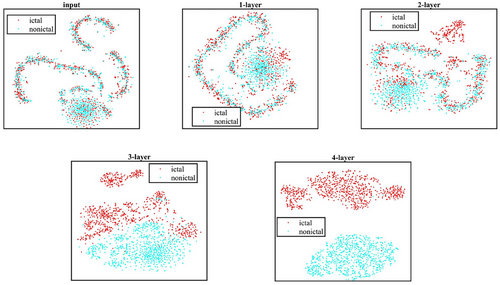
Table 10 compares the performance of our method with other seizure detection methods. Cimr et al. designed a computer-aided diagnosis (CAD) system for seizure detection based on an 8-layer CNN, utilizing built-in deep data analysis for normalization (Cimr et al. 2023). The system eliminated the need for feature extraction to reduce the complexity of the system. Ultimately, the achieved accuracy, specificity, and sensitivity were 96.99%, 96.89%, and 97.06%, respectively, which are lower than those of our method. Additionally, no event-based analysis was performed. Shyu et al. proposed a novel end-to-end deep learning model consisting of an inception module and a residual module for analyzing the multi-scale features of original EEG signals, achieving seizure detection without feature extraction (Shyu et al. 2023). The model achieved a good accuracy of 99%, but its sensitivity was lower at only 73.08%. Alharthi et al. used a new data integration and compatibility framework to solve the problem of data imbalance and used discrete wavelet transform (DWT) for preprocessing, achieving an accuracy of 96.87%, specificity of 96.98%, and sensitivity of 96.85% (Alharthi et al. 2022). Compared with our method, the overall performance of the detection method was relatively weak even using the time-consuming preprocess. Duan et al. proposed an approach to seizure detection based on deep metric learning, aiming to solve the few-shot problem by reducing the need for massive data (Duan et al. 2022). The accuracy, sensitivity, and specificity of the approach were 86.68%, 93.71%, and 79.64%, respectively, and its performance for seizure detection was not effectively improved. Li et al. developed a system using fully convolutional nested LSTM for epileptic seizure detection. Their method was tested on all cases in the CHB-MIT database, achieving a segment-based average sensitivity of 95.42%, with specificity and accuracy both at 95.29%. Under event-based evaluation, they attained a sensitivity of 94.07%, with a much higher 0.66/h FDR (Y. Li et al. 2020). Zhong et al. employed S-transform for preprocessing EEG signals and utilized a Transformer encoder as the classifier, achieving 96.11% sensitivity, 96.38% specificity, 96.15% accuracy, 96.33% F1 score, and 98.00% AUC at the segment-based level. Under event-based evaluation, their method reached a sensitivity of 96.57%, an FDR of 0.38/h. By comparison, all metrics of their model were slightly lower than those achieved by our method (Zhong et al. 2024). Dong et al. utilized the parallelism of the temporal convolutional network (TCN) and the long-range dependency mining capability of Bi-LSTM for seizure detection. Although with the strength of its simple model structure, their model delivered lower performance on both segment and event-based levels and higher FDR in comparison to our model (Dong et al. 2024).
| Author | Preprocessing method | Model | Cases | Segment-based level | Event-based level | |||||
|---|---|---|---|---|---|---|---|---|---|---|
| Accuracy (%) | Sensitivity (%) | Specificity (%) | F1 score (%) | AUC (%) | Sensitivity (%) | FDR (/h) | ||||
| Cimr et al. (2023) | CNN | 24 | 96.69 | 96.19 | 97.08 | — | ||||
| Shyu et al. (2023) | Inception and Residual module | 24 | 98.34 | 73.08 | 98.79 | — | ||||
| Alharthi et al. (2022) | DWT | 1D-CNN, Bi-LSTM, attention | 24 | 96.87 | 96.85 | 96.98 | — | |||
| Duan et al. (2022) | Deep Metric Learning | 23 | 86.68 | 93.71 | 79.64 | — | ||||
| Y. Li et al. (2020) | FC-NLSTM | 24 | 95.29 | 95.42 | 95.29 | 94.07 | 0.66 | |||
| Zhong et al. (2024) | S-Transform | Transformer | 23 | 96.15 | 96.11 | 96.38 | 96.33 | 98.00 | 96.57 | 0.38 |
| Dong et al. (2024) | TCN-BiLSTM | 24 | 97.09 | 94.31 | 97.13 | 96.48 | 0.38 | |||
| Our work | GCNN | 24 | 98.64 | 99.49 | 98.64 | 98.65 | 98.62 | 99.78 | 0.32 | |
As shown in Table 10, our model yields better performance in seizure detection when compared to other methods, enhancing its potential for real-world deployment. However, the current model is patient-specific, and cross-patient generalization remains a challenge due to variability in seizure patterns and signal characteristics. Future research will focus on addressing this variability and optimizing the system for broader applicability with a user-friendly toolbox. Additionally, further improvements in computational efficiency will enable seamless integration into handheld or wearable systems.
6 Conclusion
This study introduces a GCNN-based deep-learning framework for automated seizure detection, addressing key limitations in existing methods by incorporating the spatial relationships between EEG electrodes. By modeling these relationships as a graph structure, the GCNN captures both local and global features, enabling more precise and robust analysis of multi-channel EEG data. The system's streamlined preprocessing, lightweight design, and high accuracy make it particularly suitable for resource-constrained clinical environments.
Validation on the CHB-MIT database (pediatric patients) and the SH-SDU database (middle-aged and elderly patients) demonstrates the framework's generalizability across diverse populations. On the CHB-MIT scalp EEG database, our framework achieved an average accuracy of 98.64%, sensitivity of 99.49%, specificity of 98.64%, F1 score of 98.65%, and AUC of 98.62% at segment-based level. Under the event-based level, we recorded a sensitivity of 96.81% and FDR of 0.27/h. On the SH-SDU database, our method yielded segment-based accuracy of 95.23%, sensitivity of 92.42%, specificity of 95.25%, F1 score of 94.80%, and AUC of 95.04% along with event-based sensitivity of 94.11%. These results underscore the model's robust generalizability across diverse populations and suitability for real-world deployment, making it a promising tool for advancing epilepsy diagnostics and monitoring.
Author Contributions
Dezan Ji conceived the methodology, designed and performed the experiments, analyzed the data, and wrote the manuscript. Haozhou Cui and Haotian Li performed the experiments, analyzed the data, and modified the manuscript. Weidong Zhou conceived the methodology, designed the experiments, supervised the project, and modified the manuscript. Guoyang Liu and Yi Li analyzed the data and modified the manuscript. Zhen Liu and Wei Shang contributed data and performed the analysis. All of the authors discussed the results and reviewed the manuscript.
Conflicts of Interest
The authors declare no conflicts of interest.
Open Research
Data Availability Statement
The CHB-MIT database analyzed in this study is available at https://physionet.org/content/chbmit/1.0.0/. The SH-SDU database analyzed in this study is available from the corresponding author upon reasonable request.


