A new family of acceptable nonlinear methods with fixed and variable stepsize approach
Abstract
Solving stiff, singular, and singularly perturbed initial value problems (IVPs) has always been challenging for researchers working in different fields of science and engineering. In this research work, an attempt is made to devise a family of nonlinear methods among which second- to fourth-order methods are not only stable but acceptable as well under order stars' conditions. These features make them more suitable for solving stiff and singular systems in ordinary differential equations. Methods with remaining orders are either zero- or conditionally stable. The theoretical analysis contains local truncation error, consistency, and order of accuracy of the proposed nonlinear methods. Furthermore, both fixed and variable stepsize approaches are introduced wherein the latter improves the performance of the devised methods. The applicability of the methods for solving the system of IVPs is also described. When used to solve problems from physical and real-life applications, including nonlinear logistic growth and stiff model for flame propagation, the proposed methods are found to have good results.
1 Introduction
The emergence of nonlinear methods in solving many kinds of problems under the scalar and vector versions has intrigued many researchers to study more on this topic. Some past and recently published research work on nonlinear methods are.7-15 The analysis of ordinary differential equations is an essential tool for investigating the relationship between various dynamical quantities on which more literature can be found in Reference 16. It is challenging to find the exact solution of differential equation-based models in various situations, mainly when the problem is either nonlinear, stiff, singular, or singularly perturbed. In these conditions, we move toward the nonlinear, trigonometrically-fitted, Runge–Kutta collocation, and BDF-type Chebyshev numerical methods.17-24 After being motivated with research works recently carried out for devising or modifying nonlinear numerical methods that are suitable for stiff and singular IVPs, we attempt to derive a new family of nonlinear methods with second to the fourth-order of accuracy, and stability feature of the methods is also established. This article first derives the methods with constant step size and later formulates the proposed methods with a variable stepsize approach.
It may also be noted before starting formal analysis that whether the initial value problem (1) under consideration has a unique solution or not. The “existence” and “uniqueness” of solutions are essential things to study to solve problems and make predictions. Following the Lipschitz condition is the most frequently used criterion among various existing strategies to test the existence of a unique solution to (1).
Definition 1.The function is said to fulfill the Lipschitz condition in its dependent variable if there exists a positive constant M, commonly called the Lipschitz constant, such that for any and .
Now, the above definition can be employed in the theorem given below.
Theorem 1.Consider an IVP of the form (1) where is continuous in its independent variable and fulfills the Lipschitz condition in its dependent variable. This approach implies the existence of a unique solution to the IVP (1).
The present article is divided into seven sections as follows: In the Section 1 above, we have discussed the need to devise nonlinear numerical methods for solving IVPs with stiffness, singularities, and singularly perturbed nature. In Section 2, general formulation for the family of nonlinear methods is proposed that leads to having three nonlinear methods with stability characteristics, whereas methods with remaining orders are found to be either zero- or conditionally stable. Section 3 is concerned with the theoretical analysis of the newly devised family wherein we discuss conventional linear stability, stability with order stars, local truncation errors, and consistency of the proposed nonlinear methods. In Section 4, the applicability of the methods for system of first order ordinary differential equations is discussed. Section 5 is concerned with variable stepsize approach. In Section 6; some stiff, singular, and singularly perturbed IVPs in terms of first-order and system of first-order ordinary differential equations are taken from scientific areas to observe numerical dynamics of the proposed methods in comparison to other methods existing in the literature. In comparison to other methods, a discussion of the obtained results is carried out in the final Section 7.
2 Derivation of Proposed Methods
2.1 First-order method
It is worth noting that the method devised in (7) turns out to be the well-known forward Euler's method whose zero-stability is easy to verify. Since the method (7) is a well-established method in the available literature, therefore we will not be discussing it in detail in our research analysis. Instead, our primary focus will remain on developing nonlinear methods and possessing strong stability characteristics, making them suitable for stiff and singularly perturbed problems. Moreover, we use the notation “” that stands for the first-order linear method with zero-stability.
2.2 Second-order nonlinear method
We use the notation “” that stands for the above second-order nonlinear method with -stability.
2.3 Third-order nonlinear method
We use the notation “” that stands for the above third-order nonlinear method with -stability.
2.4 Fourth-order nonlinear method
We use the notation “” that stands for the above fourth-order nonlinear method with -stability.
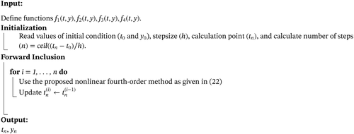
The newly proposed formulation suggested in (2) can be expanded to obtain nonlinear methods with higher-order accuracy by putting but it has been observed that the methods with and its higher values do not yield stable nonlinear methods. Therefore, we will be analyzing the nonlinear methods derived above with second-, third- and fourth-order of accuracy, that is, the methods given in (12), (17), and (22). Given below is the pseudo-code for the method given in (22). It will help readers to write the method in the programming language of their interest.
3 Theoretical Analysis
This section is dedicated to theoretical analysis of proposed nonlinear methods wherein the analysis is carried out in terms of traditional and modern stability investigations, accuracy with consistency, and the principal local truncation error term.
3.1 Stability analysis
Now, we carry out stability analysis of the proposed methods in the following theorem.
Proof.Following difference equations are obtained when the methods (12), (17), and (22) are employed on the Dahlquist's test problem (23):
Letting , following stability functions are obtained:

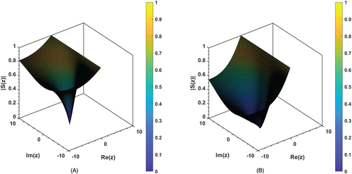
3.1.1 Stability via order stars
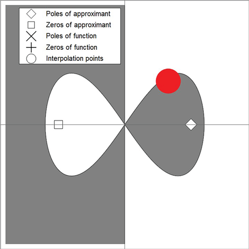
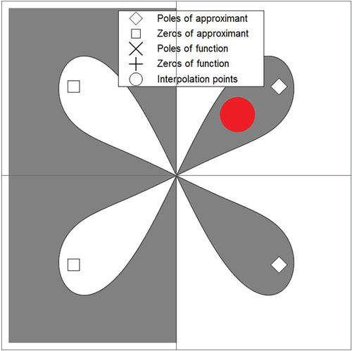
When plotted, the above sets produce star-like aspects which are somehow more anomalous than commonly known regions of absolute stability. Thus, at this stage, the concept of acceptability can be defined.
Definition 2.( acceptability) The stability function is said to be acceptable if and only if has no intersection with the imaginary axis and it possesses no poles in the left half complex plane, namely where .
In Figure 3, order stars are shown for the proposed method (12), whereas for the methods (17) and (22), the order stars are presented in Figure 4; where is represented by the shaded regions. From these figures, no intersection of is observed with the imaginary axis. In addition to this, there are no poles in the left-half of the complex plane . This shows that the rational stability functions given in (25) are acceptable with , where .
3.2 Order and consistency analysis
Thus, the newly proposed nonlinear methods (NMAS) given in (12), (17), and (22) are proved to be consistent with second-, third-, and fourth-order of accuracy.
3.3 Local truncation error analysis
Theorem 3.The nonlinear methods proposed in Equations (12), (17), and (22) have second-, third-, and fourth-order of accuracy, respectively.
Proof.The functional provided in (28) yields the following local truncation errors for the three nonlinear methods proposed:
4 Proposed Methods to Differential Systems
5 Variable Stepsize Approach
In the sections discussed above, constant stepsize approach was employed for the methods developed in (12),(17), and (22). However, it is known from the existing literature43 that a numerical method must behave accurately when stepsize h is varied. Keeping this observation in mind, we have attempted to test our developed methods under the variable stepsize approach. Now, the methods in (12),(17), and (22) can be joined with lower-order methods to perform as embedded pairs. It follows from such pairs that the numerical values utilized by lower-order methods are required to be used by higher-order methods, and this brings no additional computational cost for the method. The higher-order method is always employed to advance the integration steps once the lower-order method has been employed to estimate the local error at each step. The strategy proposed by Shampine et al.44 is adopted in the present study to design the nonlinear proposed methods under variable stepsize shape. At this stage, the procedure, as discussed in Reference 44, adopted for the variable stepsize approach is explained that depends on consideration of both the lower (p) and the higher () order methods. It may also be noted that we have considered Niekerk,45 Taylor,46 and Ramos47 methods with second-order accuracy as possible variable stepsize formulations for the Niekerk,48 Taylor,46 and the proposed methods with third-order accuracy respectively. Similarly, the Niekerk,48 Taylor,46 and Ramos49 methods with third-order accuracy are used as possible variable stepsize formulations for the Niekerk,48 Taylor,46 and the proposed methods with fourth-order accuracy respectively given in the present paper.
6 Numerical Dynamics with Results and Discussion
In this section, we have simulated several models, including nonlinear, stiff, and singular IVPs. Results obtained with the proposed second-, third-, and fourth-order convergent methods are shown in tabular form, whereas these results have been compared with the results obtained with second-order methods called the nonstandard explicit integration scheme (Ramos) taken from Reference 47 and the Taylor series method given as , third-order methods called the rational one-step method (Niekerk) taken from Reference 48 and the Taylor series method given as ; and finally with the fourth-order methods known as the rational one-step method (Niekerk) taken from Reference 48 and the Taylor series method given as . The comparison of results is based on three types of absolute errors known as the maximum absolute error computed by , the final absolute error computed by , the absolute root mean squared value computed by , and the CPU time is measured in seconds. All the numerical computations have been performed using MATLAB with version “9.8.0.1323502 (R2020a)” running on OS Windows with a processor Intel(R) Core(TM) i7-1065G7 CPU @ 1.30 GHz 1.50 GHz and installed RAM of 24.0 GB. During several simulations, the time value obtained through MATLAB on first run of the code is zero, which means that the code takes less time than the time unit used (1/100000 s.) to do the computations.
Problem 1.Consider the following nonlinear model for the kinetic behavior of biosorption:14
For the nonlinear model 1, we have shown the numerical results in Tables 1,2, and 3 with second-, third-, and fourth-order methods, respectively. It can be observed from these tables that the proposed nonlinear family of methods not only yields the smallest errors but also takes the fewest amount of CPU time (s) in most cases. It is also evident from the Tables that the second-order explicit nonstandard method (Ramos) produces results as promising as the results obtained with the second-order proposed nonlinear method. Moreover, it is also worth to be noted that the errors decrease under each method, with particularly third- and fourth-order convergence for smaller values of the stepsize h.
| Method/h | |||||
|---|---|---|---|---|---|
| Ramos | 1.2126e-03 | 3.0469e-04 | 7.6400e-05 | 1.9129e-05 | 4.7862e-06 |
| 5.7341e-09 | 1.4600e-09 | 3.6676e-10 | 9.1813e-11 | 2.2963e-11 | |
| 4.5575e-04 | 1.1472e-04 | 2.8790e-05 | 7.2119e-06 | 1.8048e-06 | |
| 1.8360e-04 | 2.8900e-04 | 7.2650e-04 | 1.3643e-03 | 2.6860e-03 | |
| Taylor | 3.2945e-04 | 8.3120e-05 | 2.0878e-05 | 5.2338e-06 | 1.3101e-06 |
| 1.0615e-08 | 2.3748e-09 | 5.6744e-10 | 1.3900e-10 | 3.4417e-11 | |
| 1.2693e-04 | 3.1626e-05 | 7.8987e-06 | 1.9740e-06 | 4.9344e-07 | |
| 1.8360e-04 | 3.0620e-04 | 7.2650e-04 | 1.3491e-03 | 2.6860e-03 | |
| 1.2126e-03 | 3.0469e-04 | 7.6400e-05 | 1.9129e-05 | 4.7862e-06 | |
| 5.7341e-09 | 1.4600e-09 | 3.6676e-10 | 9.1813e-11 | 2.2963e-11 | |
| 4.5575e-04 | 1.1472e-04 | 2.8790e-05 | 7.2119e-06 | 1.8048e-06 | |
| 1.6490e-04 | 2.8900e-04 | 7.4230e-04 | 1.3643e-03 | 2.5188e-03 |
| Method/h | |||||
|---|---|---|---|---|---|
| Niekerk | 1.3385e-04 | 2.1345e-05 | 2.8790e-06 | 3.8033e-07 | 4.9007e-08 |
| 2.7776e-10 | 1.9457e-11 | 2.4588e-12 | 3.1841e-13 | 4.2411e-14 | |
| 4.2443e-05 | 3.1035e-06 | 3.6557e-07 | 4.1214e-08 | 4.3838e-09 | |
| 4.8110e-04 | 5.9510e-04 | 1.1226e-03 | 3.3188e-03 | 2.7823e-03 | |
| Taylor | 2.7499e-05 | 3.5297e-06 | 4.4640e-07 | 5.6146e-08 | 7.0403e-09 |
| 4.7270e-10 | 5.4869e-11 | 6.6053e-12 | 8.1046e-13 | 1.0025e-13 | |
| 7.4220e-06 | 9.4883e-07 | 1.2011e-07 | 1.5115e-08 | 1.8958e-09 | |
| 4.5670e-04 | 5.5960e-04 | 8.4510e-04 | 1.8447e-03 | 2.7529e-03 | |
| 1.5565e-05 | 1.9864e-06 | 2.5104e-07 | 3.1545e-08 | 3.9538e-09 | |
| 8.8755e-12 | 1.3355e-12 | 1.8119e-13 | 2.3537e-14 | 2.8866e-15 | |
| 5.2602e-06 | 6.7436e-07 | 8.5385e-08 | 1.0742e-08 | 1.3472e-09 | |
| 3.2130e-04 | 5.1470e-04 | 8.0700e-04 | 1.2403e-03 | 2.1836e-03 |
| Method/h | |||||
|---|---|---|---|---|---|
| Niekerk | 5.8544e-07 | 3.6957e-08 | 2.3184e-09 | 1.4521e-10 | 9.0847e-12 |
| 3.8390e-12 | 2.3959e-13 | 1.4877e-14 | 9.9920e-16 | 2.2204e-16 | |
| 1.9751e-07 | 1.2474e-08 | 7.8398e-10 | 4.9139e-11 | 3.0758e-12 | |
| 2.7240e-04 | 4.8340e-04 | 1.2256e-03 | 2.4422e-03 | 3.1887e-03 | |
| Taylor | 1.0231e-06 | 6.5428e-08 | 4.1438e-09 | 2.6065e-10 | 1.6343e-11 |
| 1.7014e-11 | 9.7944e-13 | 5.8731e-14 | 3.9968e-15 | 0.0000e+00 | |
| 2.9736e-07 | 1.8831e-08 | 1.1865e-09 | 7.4477e-11 | 4.6653e-12 | |
| 2.4270e-04 | 4.0790e-04 | 9.9530e-04 | 1.6764e-03 | 4.1680e-03 | |
| 4.0982e-07 | 2.5858e-08 | 1.6248e-09 | 1.0183e-10 | 6.3731e-12 | |
| 3.6751e-12 | 2.2926e-13 | 1.4322e-14 | 9.9920e-16 | 2.2204e-16 | |
| 1.3402e-07 | 8.4866e-09 | 5.3409e-10 | 3.3499e-11 | 2.0973e-12 | |
| 2.7310e-04 | 4.7410e-04 | 8.6720e-04 | 1.8285e-03 | 3.6483e-03 |
Problem 2.Consider the following singular IVP:47
For the singular IVP 2, we have shown the numerical results in the Tables 4,5, and 6 with second-, third-, and fourth-order methods, respectively. It can be observed from these tables that the proposed nonlinear family of methods not only yields the smallest errors but also takes the fewest amount of CPU time (s). It is also evident from Tables 4,5, and 6 that Taylor's second-, third-, and fourth-order methods failed at various iterations, and the second-order explicit nonstandard method (Ramos) produces results as promising as the results obtained with the second-order proposed nonlinear method. Moreover, it is also worthy of being noted in Table 6 that the numerical results obtained under fourth-order Niekerk and the proposed method with fourth-order convergence are identical as long as . However, it is seen that the errors decrease with the proposed method () for and smaller values of the stepsize h.
| Method/h | |||||
|---|---|---|---|---|---|
| Ramos | 1.5191e+01 | 3.2714e+00 | 1.4700e+00 | 9.4682e+00 | 2.3324e+00 |
| 7.4191e-02 | 1.8418e-02 | 4.5964e-03 | 1.1486e-03 | 2.8712e-04 | |
| 4.5818e+00 | 7.2320e-01 | 2.6218e-01 | 1.0531e+00 | 1.9019e-01 | |
| 2.5172e-03 | 4.5310e-04 | 2.4541e-03 | 1.0980e-04 | 1.4560e-04 | |
| Taylor | 4.4564e+04 | Failed at | Failed at | Failed at | Failed at |
| 4.4564e+04 | |||||
| 1.3437e+04 | |||||
| 4.4522e-03 | |||||
| 1.5191e+01 | 3.2714e+00 | 1.4700e+00 | 9.4682e+00 | 2.3324e+00 | |
| 7.4191e-02 | 1.8418e-02 | 4.5964e-03 | 1.1486e-03 | 2.8712e-04 | |
| 4.5818e+00 | 7.2320e-01 | 2.6218e-01 | 1.0531e+00 | 1.9019e-01 | |
| 2.5172e-03 | 4.5310e-04 | 2.4541e-03 | 1.0980e-04 | 1.4560e-04 |
| Method/h | |||||
|---|---|---|---|---|---|
| Niekerk | 2.0259e-01 | 2.3951e-02 | 5.7313e-03 | 1.7280e-02 | 2.1441e-03 |
| 9.1369e-04 | 1.0652e-04 | 1.2843e-05 | 1.5763e-06 | 1.9523e-07 | |
| 6.1119e-02 | 5.3116e-03 | 1.0094e-03 | 1.9222e-03 | 1.7500e-04 | |
| 2.0280e-04 | 3.5780e-04 | 3.7050e-04 | 3.8430e-04 | 4.2710e-04 | |
| Taylor | 2.6337e+11 | Failed at | Failed at | Failed at | Failed at |
| 2.6337e+11 | |||||
| 7.9409e+10 | |||||
| 3.8745e-03 | |||||
| 8.3198e-03 | 5.2086e-04 | 6.2214e-05 | 9.6708e-05 | 6.0445e-06 | |
| 4.8884e-05 | 3.0607e-06 | 1.9138e-07 | 1.1962e-08 | 7.4768e-10 | |
| 2.5098e-03 | 1.1533e-04 | 1.1030e-05 | 1.0757e-05 | 4.9312e-07 | |
| 7.5300e-05 | 1.3740e-04 | 1.5950e-04 | 1.5630e-04 | 7.6900e-05 |
| Method/h | |||||
|---|---|---|---|---|---|
| Niekerk | 8.3198e-03 | 5.2086e-04 | 6.2214e-05 | 9.6706e-05 | 6.1823e-06 |
| 4.8884e-05 | 3.0606e-06 | 1.9138e-07 | 1.2175e-08 | 1.1309e-09 | |
| 2.5098e-03 | 1.1533e-04 | 1.1030e-05 | 1.0757e-05 | 5.0543e-07 | |
| 6.1972e-03 | 2.5592e-03 | 1.9988e-03 | 6.1820e-03 | 5.8807e-03 | |
| Taylor | 1.0604e+22 | Failed at | Failed at | Failed at | Failed at |
| 1.0604e+22 | |||||
| 3.1973e+21 | |||||
| 4.3795e-03 | |||||
| 8.3198e-03 | 5.2086e-04 | 6.2214e-05 | 9.6708e-05 | 6.0445e-06 | |
| 4.8884e-05 | 3.0607e-06 | 1.9138e-07 | 1.1962e-08 | 7.4768e-10 | |
| 2.5098e-03 | 1.1533e-04 | 1.1030e-05 | 1.0757e-05 | 4.9312e-07 | |
| 2.2930e-04 | 2.4120e-04 | 2.0140e-04 | 4.2750e-04 | 4.7880e-04 |
Problem 3.Consider the following nonlinear IVP for the Logistic growth:54
During the numerical solution of the nonlinear logistic growth model 3, it is observed once again that the proposed family surpasses the other methods (with the exception of Ramos) as shown in Tables 7–9 with computation of different errors and CPU time (s). For the nonlinear IVP above, third-order Taylor and Niekerk methods compete well with the proposed methods. However, the latter still maintains the smallest errors and simultaneously uses the smallest amount of CPU time. Moreover, it is also worthy of being noted in Table 9 wherein numerical results obtained under fourth-order Niekerk and proposed are identical, and this happens because the IVP under consideration is not singular, for which the proposed method () is always seen to be outperforming Niekerk.
| Method/h | |||||
|---|---|---|---|---|---|
| Ramos | 3.8270e-05 | 9.5668e-06 | 2.3916e-06 | 5.9791e-07 | 1.4948e-07 |
| 3.8270e-05 | 9.5668e-06 | 2.3916e-06 | 5.9791e-07 | 1.4948e-07 | |
| 2.0403e-05 | 5.0490e-06 | 1.2558e-06 | 3.1313e-07 | 7.8180e-08 | |
| 1.0160e-04 | 1.1590e-04 | 1.3532e-03 | 1.2258e-03 | 1.0752e-03 | |
| Taylor | 4.8470e-05 | 1.2199e-05 | 3.0599e-06 | 7.6625e-07 | 1.9172e-07 |
| 4.8470e-05 | 1.2199e-05 | 3.0599e-06 | 7.6625e-07 | 1.9172e-07 | |
| 2.6477e-05 | 6.6051e-06 | 1.6494e-06 | 4.1212e-07 | 1.0300e-07 | |
| 2.3980e-04 | 2.7460e-04 | 1.4837e-03 | 1.7237e-03 | 1.0954e-03 | |
| 3.8270e-05 | 9.5668e-06 | 2.3916e-06 | 5.9791e-07 | 1.4948e-07 | |
| 3.8270e-05 | 9.5668e-06 | 2.3916e-06 | 5.9791e-07 | 1.4948e-07 | |
| 2.0403e-05 | 5.0490e-06 | 1.2558e-06 | 3.1313e-07 | 7.8180e-08 | |
| 1.0160e-04 | 1.1590e-04 | 1.3532e-03 | 1.2258e-03 | 1.0752e-03 |
| Method/h | |||||
|---|---|---|---|---|---|
| Niekerk | 1.8128e-07 | 2.2758e-08 | 2.8509e-09 | 3.5674e-10 | 4.4617e-11 |
| 1.8128e-07 | 2.2758e-08 | 2.8509e-09 | 3.5674e-10 | 4.4617e-11 | |
| 9.5980e-08 | 1.1923e-08 | 1.4857e-09 | 1.8541e-10 | 2.3157e-11 | |
| 2.0420e-04 | 2.4790e-04 | 2.2840e-04 | 3.4440e-04 | 4.9790e-04 | |
| Taylor | 1.1906e-07 | 1.4886e-08 | 1.8610e-09 | 2.3263e-10 | 2.9076e-11 |
| 1.1906e-07 | 1.4886e-08 | 1.8610e-09 | 2.3263e-10 | 2.9076e-11 | |
| 7.1051e-08 | 8.8475e-09 | 1.1038e-09 | 1.3784e-10 | 1.7219e-11 | |
| 7.3300e-05 | 1.2200e-04 | 2.9160e-04 | 4.2530e-04 | 4.3360e-04 | |
| 3.9862e-10 | 2.4913e-11 | 1.5565e-12 | 9.7922e-14 | 3.1086e-15 | |
| 3.9862e-10 | 2.4913e-11 | 1.5565e-12 | 9.7922e-14 | 3.1086e-15 | |
| 2.1252e-10 | 1.3148e-11 | 8.1731e-13 | 5.1111e-14 | 1.5452e-15 | |
| 7.1200e-05 | 1.1620e-04 | 1.5460e-04 | 1.3540e-04 | 3.4460e-04 |
| Method/h | |||||
|---|---|---|---|---|---|
| Niekerk | 3.9862e-10 | 2.4913e-11 | 1.5568e-12 | 9.7922e-14 | 3.1086e-15 |
| 3.9862e-10 | 2.4913e-11 | 1.5568e-12 | 9.7922e-14 | 3.1086e-15 | |
| 2.1252e-10 | 1.3148e-11 | 8.1734e-13 | 5.1111e-14 | 1.5452e-15 | |
| 2.4610e-04 | 2.2560e-04 | 2.9140e-04 | 4.9450e-04 | 1.2952e-03 | |
| Taylor | 8.2151e-10 | 5.2305e-11 | 3.3002e-12 | 2.0894e-13 | 1.7764e-14 |
| 8.2151e-10 | 5.2305e-11 | 3.3002e-12 | 2.0894e-13 | 1.7542e-14 | |
| 3.8996e-10 | 2.4454e-11 | 1.5308e-12 | 9.6259e-14 | 8.7814e-15 | |
| 1.0750e-04 | 5.8740e-04 | 6.6960e-04 | 6.4600e-04 | 1.7980e-03 | |
| 3.9862e-10 | 2.4912e-11 | 1.5565e-12 | 9.7922e-14 | 3.1086e-15 | |
| 3.9862e-10 | 2.4912e-11 | 1.5565e-12 | 9.7922e-14 | 3.1086e-15 | |
| 2.1252e-10 | 1.3148e-11 | 8.1731e-13 | 5.1111e-14 | 1.5452e-15 | |
| 1.0370e-04 | 1.4810e-04 | 2.5360e-04 | 3.0590e-04 | 1.1259e-03 |
Problem 4.Consider the following stiff IVP for the flame propagation:55
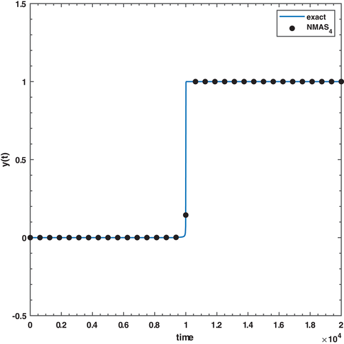
For the numerical experiment 4, we have considered an interesting model (43) of flame propagation which is a stiff ordinary differential equation as described in Reference 55. The situation illustrates that when a match is lighted, then the ball of the flame overgrows until it reaches a critical size. After that, the ball remains critical because the amount of oxygen consumed by the combustion inside the ball balances the amount of oxygen available through the surface. In model 4, the variable shows the radius of the ball, whereas the terms and stand for the surface area and the volume, respectively, at any time t. Since the initial radius, of the ball could be very small. It later varies with time. Upon comparison in Tables 10–11, the proposed third-order method () performs almost equally well as the two other third-order methods, whereas Niekerk fails when . The numerical simulations obtained with the fourth-order version of the proposed nonlinear method () are identical to the fourth-order Niekerk and Taylor results. However, the method still consumes fewer CPU seconds in most of the cases. The initial radius of the ball is taken to be during simulations. Figure 5 represents a compelling visualization of the stiff behavior of the flame propagation model that is well captured by the proposed method (). It shows that the proposed methods are adequate while dealing with the stiff models used in real-life applications.
| Method/h | |||||
|---|---|---|---|---|---|
| Niekerk | Failed at | 1.4199e-03 | 1.4199e-03 | 1.4200e-03 | 1.4200e-03 |
| 5.5511e-16 | 1.1102e-15 | 2.2204e-15 | 4.4409e-15 | ||
| 2.5701e-04 | 2.5700e-04 | 2.5700e-04 | 2.5700e-04 | ||
| 1.1144e-01 | 2.3943e-01 | 5.4002e-01 | 9.0758e-01 | ||
| Taylor | 1.4199e-03 | 1.4199e-03 | 1.4199e-03 | 1.4200e-03 | 1.4200e-03 |
| 2.2204e-16 | 4.4409e-16 | 1.1102e-15 | 2.2204e-15 | 4.4409e-15 | |
| 2.5702e-04 | 2.5701e-04 | 2.5700e-04 | 2.5700e-04 | 2.5700e-04 | |
| 7.7905e-02 | 1.3910e-01 | 2.7971e-01 | 5.7552e-01 | 1.1061e+00 | |
| 1.4199e-03 | 1.4199e-03 | 1.4199e-03 | 1.4200e-03 | 1.4200e-03 | |
| 2.2204e-16 | 5.5511e-16 | 1.1102e-15 | 2.2204e-15 | 4.4409e-15 | |
| 2.5702e-04 | 2.5701e-04 | 2.5700e-04 | 2.5700e-04 | 2.5700e-04 | |
| 8.4652e-02 | 1.3794e-01 | 2.7824e-01 | 5.7156e-01 | 1.1114e+00 |
| Method/h | |||||
|---|---|---|---|---|---|
| Niekerk | 1.4199e-03 | 1.4199e-03 | 1.4199e-03 | 1.4200e-03 | 1.4200e-03 |
| 2.2204e-16 | 5.5511e-16 | 1.1102e-15 | 2.2204e-15 | 4.4409e-15 | |
| 2.5702e-04 | 2.5701e-04 | 2.5700e-04 | 2.5700e-04 | 2.5700e-04 | |
| 3.9560e-04 | 3.2040e-04 | 3.3960e-03 | 4.3142e-03 | 3.8104e-03 | |
| Taylor | 1.4199e-03 | 1.4199e-03 | 1.4199e-03 | 1.4200e-03 | 1.4200e-03 |
| 2.2204e-16 | 5.5511e-16 | 1.1102e-15 | 2.2204e-15 | 4.4409e-15 | |
| 2.5702e-04 | 2.5701e-04 | 2.5700e-04 | 2.5700e-04 | 2.5700e-04 | |
| 9.2730e-04 | 9.6140e-04 | 3.1824e-03 | 2.3384e-03 | 6.4178e-03 | |
| 1.4199e-03 | 1.4199e-03 | 1.4199e-03 | 1.4200e-03 | 1.4200e-03 | |
| 2.2204e-16 | 5.5511e-16 | 1.1102e-15 | 2.2204e-15 | 4.4409e-15 | |
| 2.5702e-04 | 2.5701e-04 | 2.5700e-04 | 2.5700e-04 | 2.5700e-04 | |
| 2.0037e-03 | 3.5420e-04 | 1.6781e-03 | 4.0011e-03 | 2.6005e-03 |
Problem 5.Consider the following second-order IVP:49
For numerical Problem 5, we have taken a second-order IVP, or equivalently a system of two first-order differential equations wherein the singularity occurs at This singular system has been integrated over the integration interval while using the variable stepsize approach to compute the number of steps, maximum absolute error in both state variables, and the amount of time consumed by third- and fourth-order Niekerk and proposed nonlinear family of methods with variation in the tolerance values tol . It is to be noted that second-order methods are not used herein as we could not find an authentic first-order nonlinear method to be used as an embedded type pair to utilize the variable stepsize approach. It is evident from Table 12 that each third-order method yields an almost equivalent amount of maximum absolute errors. However, the Niekerk and proposed methods consume fewer steps with comparably similar consumption of CPU time (s). As far as Table 13 is concerned, the Niekerk third-order could not be successful in producing a reasonable number of steps and hence was not considered. On the other hand, the proposed nonlinear method with fourth-order convergence performs far better than its Taylor counterpart with minimum CPU time.
| Method/tol | ||||
|---|---|---|---|---|
| Niekerk | 7 | 41 | 385 | 3821 |
| 5.8246e-05 | 9.0574e-08 | 9.6490e-11 | 9.7922e-14 | |
| 1.0362e-04 | 1.4591e-07 | 1.5460e-10 | 1.5582e-13 | |
| 0 | 0 | 1.5625e-02 | 1.5625e-01 | |
| Taylor | 11 | 80 | 767 | 7640 |
| 3.0947e-05 | 3.4275e-08 | 3.4679e-11 | 4.0856e-14 | |
| 2.1424e-04 | 2.8090e-07 | 2.9043e-10 | 2.9021e-13 | |
| 0 | 0 | 3.1250e-02 | 2.9688e-01 | |
| 7 | 41 | 385 | 3821 | |
| 4.3114e-05 | 6.7921e-08 | 7.2367e-11 | 7.0388e-14 | |
| 7.7261e-05 | 1.0947e-07 | 1.1596e-10 | 1.1702e-13 | |
| 0 | 0 | 3.1250e-02 | 1.8750e-01 |
| Method/tol | ||||
|---|---|---|---|---|
| Taylor | 9 | 29 | 139 | 754 |
| 1.7932e-5 | 9.9999e-06 | 9.9999e-6 | 9.9999e-06 | |
| 1.3766e-04 | 1.3333e-05 | 1.3333e-05 | 1.3333e-05 | |
| 0 | 0 | 0 | 3.125e-02 | |
| 10 | 20 | 76 | 389 | |
| 1.7685e-05 | 3.7172e-08 | 4.6542e-11 | 5.0626e-14 | |
| 3.3606e-05 | 6.2251e-08 | 7.5484e-11 | 7.7827e-14 | |
| 0 | 0 | 0 | 1.5625e-02 |
Problem 6.Consider the following nonlinear stiff system:56
For the numerical experiment 6, a nonlinear stiff system is chosen to test the methods. The numerical results are shown in the Tables 14 and 15 reveal the tolerance values of and are enough to obtain acceptable absolute maximum errors with the smallest number of steps in most of the cases under the third and fourth-order proposed methods.
| Method/tol | ||||
|---|---|---|---|---|
| Niekerk | 41 | 250 | 2328 | 23122 |
| 8.0787e-03 | 8.8823e-05 | 8.9994e-07 | 9.0108e-09 | |
| 6.3586e-04 | 8.0051e-07 | 7.9479e-10 | 6.8512e-13 | |
| 0 | 0 | 7.8125e-02 | 1.4843 | |
| 58 | 224 | 1875 | 18384 | |
| 2.2416e-02 | 2.3796e-04 | 2.4026e-06 | 2.4069e-08 | |
| 4.8170e-04 | 4.6086e-07 | 4.8694e-10 | 4.8312e-13 | |
| 0 | 0 | 4.6875e-02 | 9.6875e-01 | |
| 30 | 239 | 2319 | 23113 | |
| 6.7037e-03 | 8.7092e-05 | 8.9816e-07 | 9.0090e-09 | |
| 7.5574e-06 | 7.5648e-09 | 7.5981e-12 | 7.4852e-15 | |
| 0 | 1.5625e-02 | 7.8125e-02 | 1.5938 |
| Method/tol | ||||
|---|---|---|---|---|
| Niekerk | 18 | 73 | 383 | 2123 |
| 9.3665e-02 | 2.8873e-03 | 9.0145e-05 | 2.8438e-06 | |
| 6.2814e-4 | 4.76e-06 | 2.8052e-08 | 1.5904e-10 | |
| 1.5625e-02 | 0 | 1.5625e-02 | 9.3750-02 | |
| 47 | 83 | 289 | 1448 | |
| 9.5727e-02 | 3.4292e-03 | 1.1480e-04 | 3.6740e-06 | |
| 3.5884e-03 | 1.8307e-05 | 1.1419e-07 | 6.5519e-10 | |
| 0 | 0 | 1.5625e-02 | 4.6875e-02 | |
| 23 | 74 | 385 | 2125 | |
| 4.1046e-02 | 2.8806e-03 | 9.0511e-05 | 2.8532e-06 | |
| 3.8977e-04 | 4.8655e-06 | 2.8183e-08 | 1.5929e-10 | |
| 0 | 0 | 1.5625e-02 | 9.3750e-02 |
Problem 7.Consider the following second-order mildly stiff nonhomogeneous IVP:57
For the numerical Problem 7, it is evident from Tables 16 and 17 that the third- and fourth-order proposed nonlinear methods perform better than the rest of the methods while consuming the same number of steps as in the Niekerk's methods but with smallest errors and comparable CPU time (s). It is worth to be noted that the fourth-order Taylor method could not compete with either method, leaving the proposed family to be the best among others taken for comparison as can be observed in Table 17.
| Method/tol | ||||
|---|---|---|---|---|
| Niekerk | 23 | 188 | 1833 | 18284 |
| 2.6046e-04 | 3.8680e-07 | 4.0732e-10 | 4.1023e-13 | |
| 2.3191e-04 | 4.6983e-07 | 5.0416e-10 | 5.0726e-13 | |
| 0 | 1.5625e-02 | 7.8125e-02 | 1.4531 | |
| 31 | 254 | 2478 | 24712 | |
| 1.1288e-04 | 1.4821e-07 | 1.5480e-10 | 1.5553e-13 | |
| 1.8117e-04 | 2.2914e-07 | 2.4365e-10 | 2.4522e-13 | |
| 0 | 1.5625e-02 | 9.375e-02 | 2.1875 | |
| 23 | 188 | 1833 | 18284 | |
| 2.2813e-04 | 3.5144e-07 | 3.7229e-10 | 3.7420e-13 | |
| 2.3372e-04 | 4.4405e-07 | 4.7339e-10 | 4.7640e-13 | |
| 0 | 0 | 9.375e-02 | 1.5781 |
| Method/tol | ||||
|---|---|---|---|---|
| Niekerk | 18 | 68 | 346 | 1910 |
| 2.6112e-04 | 3.6537e-07 | 1.2425e-09 | 1.0432e-12 | |
| 4.8810e-04 | 5.8438e-07 | 1.3439e-09 | 1.0264e-12 | |
| 0 | 0 | 3.125e-02 | 1.2500e-1 | |
| 22 | 85 | 439 | 2425 | |
| 6.0898e-05 | 3.9998e-05 | 3.9998e-05 | 3.9998e-05 | |
| 1.1999e-04 | 1.1999e-04 | 1.1999e-04 | 1.1999e-04 | |
| 0 | 0 | 1.5625e-02 | 1.0938e-01 | |
| 18 | 68 | 346 | 1910 | |
| 5.9563e-05 | 1.2362e-07 | 1.5878e-10 | 1.6766e-13 | |
| 1.2534e-04 | 2.1919e-07 | 2.6953e-10 | 2.8128e-13 | |
| 0 | 0 | 3.125e-02 | 1.2500e-01 |
7 Concluding Remarks
A new family of nonlinear numerical methods proposed in the present research study is proved to be suitable for dealing with nonlinear, stiff, and singular differential equations' based models. Three members of the proposed family having an order of convergence , and 4 are shown to be both stable and acceptable. Consistency and order of convergence with analysis of local truncation errors are well established, wherein the methods are equally applicable for systems of ordinary differential equations. The variable stepsize approach is used for nonlinear, stiff, and singular systems to obtain the smallest absolute errors with the proposed family. Real-life applications, including nonlinear logistic growth and stiff models describing the dynamical behavior of flame propagation, are successfully dealt with by the methods proposed. It would be interesting to devise, in future studies, a new class of numerical methods with multiple steps and an stability feature.
Notations
-
- h
-
- Stepsize
-
- tol
-
- Tolerance
-
- A− stability
-
- Absolute stability
-
- hini
-
- Initial stepsize
-
- RMS
-
- Root mean squared error
-
- LMZS1
-
- First-order linear method with zero-stability
-
- NMAS2
-
- Numerical method with acceptability having second-order accuracy
-
- NMAS3
-
- Numerical method with acceptability having third-order accuracy
-
- NMAS4
-
- Numerical method with acceptability having fourth-order accuracy
-
- Ramos2
-
- Explicit nonstandard second order method
-
- LTE
-
- Local truncation error
-
- est
-
- Estimate error
-
- len
-
- Local error
ACKNOWLEDGMENTS
The first and second authors are grateful to Mehran University of Engineering and Technology, Jamshoro, Pakistan, for the kind support and facilities to carry out this research work. The first author is also grateful to the Department of Mathematics, Near East University, Cyprus, including the third author.
Author Contributions
Sania Qureshi: Conceived of the idea, derived the proposed nonlinear methods, and performed numerical simulations. Amanullah Soomro: Carried out theoretical analysis of each proposed method. Evren Hınçal: Carried out supervision of the entire work. All author equally contributed toward writing and finalizing the article.
Biographies

Dr. Sania Qureshi was born in Hyderabad in 1982. S. Qureshi completed her PhD in 2019 from University of Sindh. During PhD, she was awarded two scholarships under which she visited Division of Mathematics, University of Dundee, Scotland, UK in 2016 and Institute of Computational Mathematics, Technische Universitaet Braunschweig, Germany in 2018. She has several publications on mathematical epidemiology, fractional calculus, and numerical techniques for ODEs. Since 2008, she is the full-time faculty member at Mehran University of Engineering and Technology, Pakistan.

Mr. Amanullah Soomro was born in Umerkot in 1995. In 2019, A. Soomro graduated from Institute of Mathematics and Computer Sciences, University of Sindh, Jamshoro with BS degree. Nowadays, he is pursuing M.Phil research studies from the department of Basic Sciences and Related Studies at Mehran University of Engineering and Technology, Jamshoro, Sindh, Pakistan. He is the co-author of two research papers recently published in Scopus international journals. At the same time, A. Soomro is serving as a Teaching Assistant in the same department.

Prof. Dr. Evren Hınçal was born in Lefkoşa in 1973. In 1991, E. Hınçal completed his PhD at the Eastern Mediterranean University with the cooperation of Imperial College. Between the years 2000 and 2001 E. Hınçal visited Imperial College and he worked with Neurobiology Group on the cancer epidemiology. E. Hınçal has several publications about cancer statistics, cancer epidemiology and mathematical modeling about cancer in refereed international journals. Since 2007, he is the full-time member of Near East University Department of Mathematics.


