

A collection of efficient tools to work with almost strictly sign regular matrices
Abstract
In this work, several algorithms have been implemented with Matlab to obtain an algorithmic characterizations of almost strictly sign regular matrices using Neville elimination.
1 INTRODUCTION
Numerical methods adapted to the structure of several classes of matrices has been an important field of research in recent years. A class of structured matrices very important by its applications is provided by the class of sign regular (SR) matrices, which have all minors of the same order with the same sign. The potential applicability of nonsingular SR matrices comes from their characterization as variation diminishing linear transformations, of great importance in many applications to mathematics, statistics, economy, or computer aided geometric design, among other fields (see References 1-3).
A very important subclass of SR matrices is formed by totally positive (TP) matrices, which are matrices with all their minors nonnegative. A systematic study of TP matrices starts with the work by Schoenberg in 1930 , where this definition was first introduced (see Reference 4). Krein and Gantmacher referred to these matrices as completely nonnegative matrices. Nowadays, there are several denominations for this concept. Here we use TP for matrices whose minors are nonnegative, although other authors call them totally nonnegative matrices (see Reference 5). A deep research on TP matrices can be seen in books written decades ago, such as the book by Gantmacher and Krein, whose first edition in Russian language was published in 1941 and it has an English version of 2002,6 or Karlin's book of 1968.7 Later books are the book edited by Gasca and Micchelli in 19968 and, more recently, Pinkus' book of 20099 and the book by Fallat and Johnson of 2011.10 An influential survey was published by Ando in 1987,1 where he presented many results under a linear algebra view point. In contrast, knowledge on SR matrices is comparatively scarce, due to the greater difficulties arising from their study.
Our aim is the study of another class of SR matrices formed by the almost strictly sign regular (ASSR) matrices. These matrices, introduced in 2012,11 are matrices such that all their nontrivial minors of the same order have the same sign. They generalize the class of nonsingular almost strictly totally positive (ASTP) matrices, introduced in 1992 by Gasca, Micchelli and Peña in Reference 12, which are nonsingular TP matrices such that all their minors formed by consecutive rows and columns are positive if and only if their diagonal entries are positive. Important examples of nonsingular ASTP matrices are provided by the Hurwitz matrices and B-spline collocation matrices. Alternative approaches to ASTP matrices have been developed by Adm et al.13-16
The results presented in this work include several algorithms that allow us to characterize, in an efficient way, ASSR matrices by using their Neville elimination (NE). This research field contains works characterizing SR, TP, or ASTP matrices by NE (see References 12, 17-22).
NE is an alternative elimination method to Gauss elimination and has been very useful when working with SR matrices and their subclasses. Recently some authors, including Alonso, Cortés, Delgado, Gallego, Gasca, Michelli, Mühlbach, and Peña, have carried out a systematic study of this kind of matrices with NE. Starting with Aitken-Neville interpolation formula, Gasca and Mühlbach introduced in References 21, 23 NE because this procedure arises when the Neville interpolation strategy is used to solve the corresponding linear system, analogously as happens with Gauss elimination when the Aitken interpolation strategy is used to solve it. In Reference 19, very nice properties of using NE for TP matrices were shown.
In Reference 17, a characterization of ASSR matrices by the pivots of NE was presented. The corresponding computational cost can be reduced when dealing with some subclasses of matrices, such as almost strictly totally negative or M-banded matrices (see References 17, 24, 25).
In this work, an algorithmic characterization of ASSR matrices by NE is presented. For this, several algorithms (functions) have been implemented using Matlab. The article is organized as follows. Section 2 includes basic concepts and algorithms related to type-I or type-II staircase matrices. Section 3 presents the algorithms corresponding to the characterization of the matrices.
2 BASIC CONCEPTS
For , with , denotes the set of all increasing sequences of k natural numbers not greater than n. If A is a real matrix and , , then is by definition the submatrix of A containing rows and columns of A. In particular, when , is the corresponding principal submatrix. Besides, denotes the set of increasing sequences of k consecutive natural numbers not greater than n and if , then is a principal minor.
Definition 1.A real matrix is called type-I staircase matrix if it satisfies simultaneously the following conditions:
- (a)
, ;
- (b)
, if , ;
- (c)
, if , .
Definition 2.A matrix A is called type-II staircase if is a type-I staircase matrix.
To work with a type-II staircase matrix, we consider the auxiliary matrix and apply all the procedures to it:
-
function [A Pn Type2] = Check_Type2(A,n)
-
% This function check if the matrix A has elements a_11 or a_nn equal zero,
-
% in this case, the matrix can not be staircase type I and then it can be
-
% only staircase type II, so it returns P_n*A in order to apply the type I
-
% algorithms to this matrix.
-
% Input arguments:
-
% A ……. a square matrix
-
% n …….. the order of the matrix A (optional)
-
% Output arguments:
-
% A …….. the candidate matrix to be staircase type I A or P_n*A
-
% P_n …… the backward identity matrix
-
% Type2 …. 1 if the function performs the transformation P_n*A
-
if nargin < 2; n = size(A,2); end
-
Pn = 0;
-
Type2 = 0;
-
if A(1,1) == 0 || A(end,end) == 0
-
Pn = eye(n);
-
Pn = Pn(end:-1:1,:);
-
A = Pn*A;
-
Type2 = 1;
-
end
Conditions introduced in Definitions 1 and 2 produce a staircase structure for the zero pattern, which is set through the following indices (see References 17, 26):
To obtain these indices we have these two functions:
The first function gives a vector indicating the last element of the corresponding column different from zero and check that the rest of elements are zeros.
-
function [s1,s0] = Check_Lower_Shadow(A,n)
-
% Function which computes the number of elements different from zero
-
% of each column and check that the matrix is staircase type I with
-
% 1's above the main diagonal
-
% Input arguments:
-
% A …….. a matrix with 1's or 0's
-
% n …….. the number of columns of the matrix A (optional)
-
% Output arguments:
-
% s1 …… a vector with the number of elements
-
% different from zero of each column
-
% s0 …… 0 if A is staircase Type 1 bellow the main diagonal
-
if nargin < 2; n = size(A,2); end
-
s1 = sum(A);
-
s0 = 0;
-
if ∼(all(s1(1:end-1) <= s1(2:end))); s0 = 1;end
-
for k=1:n;
-
s0 = sum([s0;A(s1(k)+1:end,k)]);
-
end
Example 1.Given the matrix A, we generate the matrix with ones above the main diagonal and in the main diagonal and bellow it the element is 1 if and 0 if it is zero.
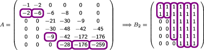
Then we apply the function to .
-
≫ [s1,s0] = Check_Lower_Shadow(B_2)
The second function gives the indices defined in (1)–(3).
-
function [I,J,s1,s0] = Find_Lower_Pattern(A,n)
-
% Function which finds the lower zero pattern of a matrix A
-
% Input arguments:
-
% A …… a square matrix
-
% n ……. the order of the matrix A (optional)
-
% Output arguments:
-
% I ……. lower zero pattern vector I=(i_0,i_1,…,i_s)
-
% J ……. lower zero pattern vector J=(j_0,j_1,…,j_s)
-
% s1 …… a vector with the row index of the last element
-
% different from zero of each column
-
% s0 …… 0 if A is staircase Type 1 bellow the main diagonal
-
if nargin < 2; n = size(A,2); end
-
B = (A==0);
-
B = tril(B);
-
B2 = 1-B;
-
[s1,s0] = Check_Lower_Shadow(B2,n);
-
s2 = sum(B.');
-
I = union(0,s1)+1;
-
J = union(s2,n)+1;
Example 2.Given A the matrix of the Example 1, the output of the command
-
≫ [I,J,s1,s0] = Find_Lower_Pattern(A)
To obtain we only need to find the I and J of the transpose, so:
-
function [I,J,Ih,Jh,s1,st1] = Find_Pattern(A,n)
-
% Function which finds the zero pattern of a matrix A
-
% Input arguments:
-
% A …….. a square matrix
-
% n …….. the order of the matrix A (optional)
-
% Output arguments:
-
% I …….. lower zero pattern vector I=(i_0,i_1,…,i_s)
-
% J …….. lower zero pattern vector J=(j_0,j_1,…,j_s)
-
% Ih ……. upper zero pattern vector Ih=(ih_0,ih_1,…,ih_r)
-
% Jh ……. upper zero pattern vector Jh=(jh_0,jh_1,…,jh_r)
-
% s1 ……. a vector with the row index of the last element
-
% different from zero of each column
-
% st1 …… a vector with the column index of the last element
-
% different from zero of each row
-
% if A is NOT staircase type I then I,J,Ih,Jh,s1,st1 will be []
-
if nargin < 2; n = size(A,2); end
-
[I,J,s1,s0] = Find_Lower_Pattern(A);
-
[Jh,Ih,st1,st0] = Find_Lower_Pattern(A.');
-
if s0 ∼= 0 || st0 ∼= 0
-
I = []; J = []; Ih = []; Jh = []; s1 = []; st1 = [];
-
end
This function also returns the vectors and which are useful for others algorithms (functions). If the matrix is not staircase then the function returns the empty set for all variables [].
Example 3.Given A the matrix of the Example 1, the output of the command
-
≫ [I,J,Ih,Jh,s1,st1] = Find_Pattern(A)
Now, we highlight some entries of the matrix of the Example 1 in two different ways
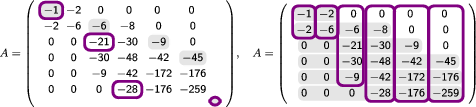
In the first representation, the framed numbers correspond with the positions given by the lower zero pattern and the numbers with grey background correspond with the positions given by the upper zero pattern (which is the lower zero pattern of the transpose). In the second representation, it can be observed the interpretation of the vectors and .
So, if A is a type-II staircase matrix, then the zero pattern of A is the zero pattern of .
To mark the positions of the matrix in which a new echelon starts, we define the following indices.
To find theses indices we have implemented the next function:
-
function [it jt] = Find_jt(i,j,I,J)
-
% Given a matrix A of order n with zero pattern I J and two numbers i, j
-
% such that 1<=j<=i<=n this function returns the indices i_j and j_t
-
% Input arguments:
-
% i …….. row position of the element a_ij
-
% j …….. column position of the element a_ij
-
% I …….. lower zero pattern vector I=(i_0,i_1,…,i_s)
-
% J …….. lower zero pattern vector J=(j_0,j_1,…,j_s)
-
% Output arguments:
-
% it ……. the index i_t
-
% jt ……. the index j_t
-
k = find(j<J,1);
-
t = find(j-i <= J(1:k-1)-I(1:k-1),1,'last');
-
it = I(t); jt = J(t);
Example 4.Given A the matrix of the Example 1, the output of the command
-
≫ [it jt]=Find_jt(5,4,I,J)
-
≫ [it jt]=Find_jt(6,6,I,J)
-
≫ [it jt]=Find_jt(5,3,I,J)
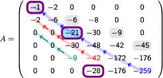
The geometrical interpretation of this concept is the following, we fix the position and draw the diagonal that passes through this position (); starting at this position, to the left, is the first position of the lower zero pattern which lies above this diagonal. In the next graph we can observe this interpretation
3 ALMOST STRICTLY SIGN REGULAR MATRICES
Next, we define ASSR matrices, which are matrices whose nontrivial minors of the same order have all the same strict sign. To store the sign we are going to define the vector of signatures.
Definition 3.Given a vector , we say that is a signature sequence, or simply, is a signature, if for all .
ASSR matrices form a subclass of SR matrices. A matrix is SR if all its minors of the same order have the same sign. That is:
Definition 4.A real matrix is said to be SR, with signature , if all its minors satisfy that
In a staircase matrix there are some minors which are trivially zero due to the position of their zero entries. We are going to distinguish those minors from those that do not verify that condition.
Definition 5.Let be a type-I (type-II) staircase matrix. A submatrix , with , is said to be nontrivial if all its main diagonal (secondary diagonal) elements are nonzero.
The minor associated to a nontrivial submatrix () is called nontrivial minor ().
The nontrivial minors play an important role in ASSR matrices.
Definition 6. ([11])A real matrix type-I or type-II staircase is said to be ASSR, with signature , if all its nontrivial minors satisfy that
Remark 1.Observe that an ASSR matrix is SR, since the trivial minors are zero and the nontrivial minors satisfy the strict inequality (9). Observe also that an ASSR matrix is nonsingular.
Next, we present the characterization given in Reference 11 for ASSR matrices (see theorem 10).
Theorem 1.Let A be a real matrix and be a signature. Then A is ASSR with signature if and only if A is a type-I or type-II staircase matrix, and all its nontrivial minors with , , satisfy
A characterization of the ASSR matrices using the pivots of NE is given in Reference 17. To carry out the Neville process (see Reference 19), we have implemented the following algorithm:
-
function [A Piv Ak] = Neville(A,n)
-
% Function to apply the Neville elimination method to a square matrix.
-
% Input arguments:
-
% A …….. a square matrix
-
% n ……… the order of the matrix A (optional)
-
% Output arguments:
-
% A ……… the matrix we obtain at the end of the process
-
% Piv ……. Matrix with the pivots of the NE algorithm
-
% Ak …….. A 3-dimensional array with all the matrices A_k
-
% of the procedure A_1=Ak(:,:,1), A_2=Ak(:,:,2),…
-
if nargin < 2; n = size(A,2); end
-
Piv = zeros(n,n);
-
for j = 1:n
-
Ak(:,:,j) = A;
-
[I,bnd] = Pivoting(A(j:end,j),j,n);
-
A = A(I,:);
-
Piv(j:end,j) = A(j:end,j);
-
for i = bnd:-1:(j+1)
-
A(i,:) = A(i,:)-A(i,j)/A(i-1,j)*A(i-1,:);
-
end
-
end
For simplicity we obtain a function to apply the pivoting strategy, that is, by moving to the bottom the rows with a zero entry:
-
function [I bnd] = Pivoting(v,j,n)
-
% Function to apply pivoting strategy
-
% Input arguments:
-
% v ……… a column vector with the elements (a_jj,a_{j+1j},…,a_nj)
-
% j …….. index of the column we are applying the method
-
% n ……… order of the matrix
-
% Output arguments:
-
% I ……… the new order to put the zero entries down
-
% bnd ……. the position of the last element different from zero
-
vv = ones(n,1);
-
vv(j:n) = abs(v)/max(abs(v)) ∼= 0;%We can use (>10∧k*eps) instead of (∼=0)
-
[vv I] = sort(vv,'descend');
-
bnd = find(vv,1,'last');
Although all the output arguments are not necessary, the function returns the final matrix, all the intermediate matrices and the pivots of the process with the realignment.
This characterization uses the following results:
Theorem 2.Let be a nonsingular type-I staircase matrix, with zero pattern defined by I, J, , and . If B is ASSR with signature , then the NE of B can be performed without row exchanges and the pivots satisfy, for ,
Theorem 3.Let be a nonsingular type-II staircase matrix, with zero pattern defined by I, J, , and . If B is ASSR with signature , then the NE of can be performed without row exchanges and the pivots satisfy, for ,
Remark 2.Using this theorems it is easy to verify that and
To check the pivot conditions of Theorem 2 we have implemented the function:
-
function PSignat = Check_p_ij_Cond(Piv,s1,PSignat,n)
-
% This function check that the pivots Piv of the Neville Elimination of
-
% a matrix A verifies the conditions:
-
% ep_{j-1}*ep_j*p_ij > 0 if a_ij ∼= 0 and p_ij == 0 if a_ij == 0
-
% Input arguments:
-
% Piv ……. matrix with the pivots of the NE of the matrix
-
% s1 …….. a vector with the row index of the last element
-
% different from zero of each column
-
% PSignat … vector with the products of consecutive elements (optional)
-
% of the signature (ep_0*ep_1,ep_1*ep_2,….,ep_{n-1}*ep_n)
-
% PSignat = [sign(p_11),sign(p_22),…,sign(p_nn)]
-
% n ……… the order of the matrix (optional)
-
% Output arguments:
-
% PSignat …. PSignat if the conditions are verified or 0 otherwise
-
if nargin < 4; n = size(Piv,2); end; if nargin < 3; PSignat=[]; end;
-
if isempty(PSignat)
-
PSignat = sign(diag(Piv)).';
-
elseif PSignat == 0
-
return
-
end
-
M = Piv*diag(PSignat(1:n));
-
for j = 1:n
-
if ∼all(M(j:s1(j),j) > 0); PSignat = 0; return;end
-
end
If we want to verify the conditions of Theorem 3, it is enough to apply the previous function the matrix .
From now on, we will denote by . Note that and .
Remark 3.Let A be a type-I (type-II) staircase matrix. Then, in relation to () matrices, the next results are verified:
- and are also type-I (type-II) staircase matrix for all .
- If the zero pattern of A is given by , , , , then the zero pattern of matrices is given by , , , , where and .
- If A is ASSR matrix with signature then and are ASSR matrices with signature .
To obtain the zero pattern of the matrices from the zero pattern of A we have the function:
-
function [I_h J_h] = Lower_Zero_Pattern_Of_A_h(I,J,h)
-
% Given a matrix A with zero pattern I J this function returns the lower
-
% zero pattern of the submatrix A_h
-
% Input arguments:
-
% I ……… lower zero pattern vector I=(i_0,i_1,…,i_s)
-
% J ……… lower zero pattern vector J=(j_0,j_1,…,j_s)
-
% h ……… index of the matrix A_h we are checking
-
% Output arguments:
-
% I_h ……. lower zero pattern vector I_h of A_h
-
% J_h ……. lower zero pattern vector J_h of A_h
-
I_h = I-h+1; J_h = J-h+1;
-
J_h = [1 J_h(J_h > 1)];
-
hh = length(J_h);
-
I_h = [1 I_h(end-hh+2:end)];
By checking the compatibility of the signature needed for the last condition of the previous result, we need only a function to check bellow the main diagonal because to check above the main diagonal we can apply this one to the transpose, that is:
-
function PSignat = Check_Signature_Lower_Compatibility(I,J,h,PSignat)
-
% Given a matrix A with zero pattern I J, we study the compatibility of the
-
% signature for the indices of the submatrices A_h bellow the main diagonal,
-
% that is, if i∧h >= j∧h and i∧h - j∧h == i∧h_t - j∧h_t then
-
% ep_{j∧h - j∧h_t}·ep_{j∧h - j∧h_t+1} ==ep_{j∧h - 1}·ep_{j∧h}
-
% Input arguments:
-
% I ……… lower zero pattern vector I=(i_0,i_1,…,i_s)
-
% J ……… lower zero pattern vector J=(j_0,j_1,…,j_s)
-
% h ……… index of the matrix A_h we are checking
-
% PSignat … vector with the products of consecutive elements of
-
% the signature (ep_0*ep_1,ep_1*ep_2,….,ep_{n-1}*ep_n)
-
% Output arguments:
-
% PSignat … PSignat if the conditions are verified or 0 otherwise
-
if PSignat == 0; return; end
-
[I J] = Lower_Zero_Pattern_Of_A_h(I,J,h);
-
n = (I(end)-1);
-
IJ = [I(2:end-1); J(2:end-1)];
-
for ij = IJ
-
for i = ij(1):n
-
j = ij(2) + i - ij(1);
-
[it jt] = Find_jt(i,j,I,J);
-
if (i-j == it-jt) && PSignat(j-jt+1) ∼= PSignat(j)
-
PSignat = 0; return;
-
end
-
end
-
end
Finally, in the following result (theorem 5 of Reference 17) a characterization of ASSR matrices, with , is presented:
Theorem 4.A nonsingular matrix is ASSR with signature , with if and only if for every the following properties hold simultaneously:
- a)
A is type-I staircase;
- b)
the NE of the matrices and can be performed without row exchanges;
- c)
the pivots of the NE of satisfy conditions corresponding to (12), (13), and the pivots of the NE satisfy (14) and (15);
- d)
for the positions of matrix :
-
if and then ,
- if and then ,
where indices are given by conditions corresponding to (7) and (8).
-
The final function, which computes the signature and return it if the matrix is ASSR using this characterization theorem is:
-
function Signat = Signature(A)
-
% Function to check if a matrix A is ASSR, if so, finds the signature
-
% Input arguments:
-
% A ……… an square matrix
-
% Output arguments:
-
% Signat …. the signature of A if it is ASSR, 0 otherwise.
-
n = size(A,1);
-
Signat = [];
-
[A Pn Type2] = Check_Type2(A,n);
-
[I,J,Ih,Jh,s1,st1] = Find_Pattern(A,n);
-
if isempty(I); Signat = 0; return; end
-
for h = 1:n
-
A_h = A(h:end,h:end);
-
[B Piv Ak] = Neville(A_h,n-h+1);
-
Signat = Check_p_ij_Cond(Piv,s1(h:end)-h+1,Signat,n-h+1);
-
Signat = Check_Signature_Lower_Compatibility(I,J,h,Signat);
-
if Signat == 0; return; end
-
[Bt Piv Ak] = Neville(A_h.',n-h+1);
-
Signat = Check_p_ij_Cond(Piv,st1(h:end)-h+1,Signat,n-h+1);
-
Signat = Check_Signature_Lower_Compatibility(Jh,Ih,h,Signat);
-
if Signat == 0; return; end
-
end
-
[A Signat] = Recover_A_And_Obtain_Signature(A,Signat,Pn,Type2,n);
-
end
An auxiliary function we use in the function Signature is defined bellow:
-
function [A Signat] = Recover_A_And_Obtain_Signature(A,PSignat,Pn,Type2,n)
-
% This is an auxiliary function of the Signature function, in the signature
-
% function we work with the vector PSignat and with this function we
-
% recover the signature vector and, if the matrix is staircase type II then
-
% we apply the signs relationship to obtain the Signature
-
% Input arguments:
-
% A …….. a square matrix
-
% PSignat … vector with the products of consecutive elements
-
% of the signature (ep_0*ep_1,ep_1*ep_2,….,ep_{n-1}*ep_n)
-
% P_n ……. the backward identity matrix
-
% Type2 ….. 1 or 0
-
% n ……… the order of the matrix A (optional)
-
% Output arguments:
-
% A ……… A or Pn*A
-
% Signat …. the signature of A if it is ASSR, 0 otherwise.
-
if nargin < 2; n = size(A,2); end
-
Signat(1)=PSignat(1);
-
for i = 2:n
-
Signat(i) = Signat(i-1)* PSignat(i);
-
end
-
if Type2 == 1
-
i = 1:n;
-
k = i.*(i-1)/2;
-
A = Pn*A;
-
Signat = Signat.*[(-1).∧k];
-
end
-
end
Next, a simple example to show the efficiency of the function Signature is presented.
Example 5.Given the matrices
-
≫ epsilon = Signature(M)
-
≫ epsilon = Signature(N)
The second matrix fails because, as we know, the matrix is staircase type II so we must to multiply by the identity backward matrix and apply the Theorem 4 to . So the NE process of the matrices and throws these pivots
The pivot and it must be negative.
We finish with a interesting example:
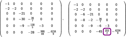
Example 6.Let A be the matrix
Now, if we apply the function Neville to and , the pivots and and the signs of the pivots are,
ACKNOWLEDGMENT
This work has been partially supported by the Spanish Research Grants PGC2018-096321-B-I00, TIN2017-87600-P, MTM2017-90682-REDT and by Gobierno de Aragón (E41_20R).
Biographies

Pedro Alonso Velázquez received the M.Sc degree in Mathematical Sciences, from the University of Zaragoza (Spain) and the Ph.D. degree in Mathematical Sciences (Cum Laude) at the University of Oviedo (Spain). Currently, he is a full professor in Applied Mathematics at the University of Oviedo. His research areas are framed in the Numerical linear algebra, error analysis, study of algorithms (complexity, performance, stability, convergence, error, etc.), as well as in different aspects of fuzzy logic.

Jorge Jiménez Meana received the M.Sc degree in Mathematical Sciences, from the University of Salamanca (Spain) and the Ph.D. degree in Mathematical Sciences (Cum Laude) at the University of Valladolid (Spain). Currently, he is professor in Applied Mathematics at the University of Oviedo. His research areas are framed in the Numerical linear algebra, parallel algorithms, cryptography, and algebraic structures in fuzzy sets.

Juan Manuel Peña Ferrández is a Full Professor at the Department of Applied Mathematics of the University of Zaragoza (Spain). He received a M.Sc degree and a Ph.D. degree in Mathematical Sciences from the University of Zaragoza. He is author of more than 300 published research papers. His current research interests are Numerical Linear Algebra, Total Positivity, Nonnegative Matrices, Structured Matrices, Numerical Analysis, Approximation Theory, Shape Preservation and Computer-Aided Geometric Design.

María Luisa Serrano Ortega received the M.Sc degree in Mathematical Sciences, from the University of Valencia (Spain) and the Ph.D. degree in Mathematical Sciences (Cum Laude) at the University of Oviedo (Spain). Currently, she is professor in Applied Mathematics at the University of Oviedo. His research areas are framed in the Numerical linear algebra.

