A block preconditioner for two-phase flow in porous media by mixed hybrid finite elements
Funding information: Qatar National Research Fund, NPRP10-0208-170407
Abstract
In this work, we present an original block preconditioner to improve the convergence of Krylov solvers for the simulation of two-phase flow in porous media. In our modeling approach, the set of coupled governing equations is addressed in a fully implicit fashion, where Darcy's law and mass conservation are discretized in an original way by combining the mixed hybrid finite element (MHFE) and the finite volume (FV) methods. The solution to the sequence of large-size nonsymmetric linearized systems of equations that stem during a full-transient simulation represents the most time and resource consuming task, thus motivating the need for efficient preconditioned Krylov solvers. The proposed preconditioner exploits the block structure of the Jacobian matrix while coping with the nonsymmetric nature of the individual blocks. Both academic and realistic applications have been used to challenge the preconditioner, allowing to point out its robustness, stability and overall computational efficiency.
1 INTRODUCTION
Solving series of large-size sparse systems of equations is a key task for modeling transient physical processes, often posing an issue in terms of high computational cost. The target of this paper is the efficient solution of the linear(ized) systems of equations originating from the simulation of two-phase flow in porous media, which is a classical fundamental application for the energy industry. Despite the continuous development of computer hardware technology with ever more powerful processing units and larger memory capacities being released, high runtime and storage demand are frequent drawbacks encountered in reservoir modeling due to the increase of model size for more accurate simulations. The solving procedure, and hence the linear solver, is usually the main responsible for that. In typical reservoir simulations, around 60% to 80% of the total CPU time is spent in this task.1, 2
The flow of two fluid phases in porous media is governed by the mass balance equations coupled with Darcy's law. In our modeling approach, the weak formulation of this set of PDEs is obtained by applying the Finite Volume (FV) method with a low-order time-marching scheme to the continuity equations and the Mixed Hybrid Finite Element (MHFE)3 method to Darcy's law. The FV method is a well-established choice in reservoir simulations, since it guarantees the mass conservation both at the local and global level, that is, a primary requirement in transport-based problems. On the other hand, a number of schemes can be found in literature for the discretization of Darcy's law. The most popular one is perhaps the simple two-point flux approximation (TPFA),4 which, however, suffers from well-known limitations in dealing with full tensor rock-fluid properties and unstructured grids. Its extension, the multi-point flux approximation (MPFA) variant,5-7 is another popular strategy along with the mimetic finite difference (MFD) scheme, which has been recently used in a two-phase flow model in fractured media.8 Nevertheless, the approximation accuracy in determining the fluid pressure and velocity, even on unstructured meshes with full tensor medium properties, and the continuity of the normal component of the fluxes through the interfaces of the grid, while honoring the mass conservation at the element level,9, 10 have made the MHFE an alternative robust approach. Despite a few drawbacks, such as the enlargement of the stencil or the breach of the discrete maximum principle,11 MHFE and the pioneering nonhybridized version, the mixed finite element (MFE) method, have witnessed an increasing popularity in the last decade. Recent significant applications include coupled flow-poromechanics,12-16 deformation models,17, 18 multiphase19-23 and coupled Stokes–Darcy24 flow in porous media. An MHFE discretization of the two-phase flow model in porous media, which is similar to the one introduced in this work, was proposed by Fučík and Mikyška,25 but it relied on a sequential splitting technique to handle the inherent coupling of the governing equations. In our modeling approach, instead, the coupled solution is addressed by an unconditionally stable fully implicit approach, whereas the inherent nonlinearity is dealt with a Newton scheme, which requires at each time step the solution to a sequence of linearized systems of equations with the Jacobian matrix. Since such systems are usually very large (i.e., unknowns and more) and ill-conditioned, iterative techniques, and specifically preconditioned Krylov subspace methods,26 are necessary for their solution.
In order to attain a fast convergence, Krylov subspace solvers need to be equipped with robust and efficient preconditioners that should take advantage of the Jacobian block structure. In this regard, multistage preconditioners, such as the constrained pressure residual (CPR),27, 28 are the standard for industry reservoir simulators. In its basic structure, the two-stage multiplicative CPR algorithm couples an AMG preconditioner for the usually elliptic pressure block and an incomplete factorization for the full matrix. The popularity of this scheme is mostly related to the high scalability of AMG, which is tailored for elliptic problems. The classical version of the CPR preconditioner, however, does not prove highly effective for the MHFE-FV-discretized two-phase flow model, since it is not capable to capture the composite structure of the nonsymmetric pressure block, resulting from the introduction of pressure unknowns on both elements and faces. Such a submatrix exhibits, in fact, an inner block structure, that can be well exploited by means of a block preconditioning strategy. Although block preconditioners have found some application in reservoir simulators only in recent years,29 they have been long developed for other problems,30 such as the solution of the Navier–Stokes equations,31, 32 coupled poromechanics,33-35 electromagnetism,36, 37 and contact mechanics,38-40 just to cite some.
Specific preconditioners have been also developed in the past for the two-phase flow problem in porous media. Bergamaschi et al.41 developed a preconditioning technique upon a finite element discretization of the governing equations. The preconditioner consists of an incomplete factorization of the whole Jacobian matrix which is repeatedly updated during the simulation. More recently, Skogestad et al.42 followed a different approach by designing an ASPIN-like43 nonlinear preconditioner based on a TPFA approximation of Darcy's equation. Nonlinear preconditioners operate at the level of the nonlinear problem, with a different approach than the linear stage. To the best of our knowledge, this work is one of the first attempts to design a full block preconditioner for the two-phase flow problem in porous media discretized by a combined MHFE-FV strategy.
The rest of the paper is organized as follows. In Section 2 the set of equations governing the two-phase flow in porous media is presented along with the numerical formulation. Our block preconditioner is then introduced and tested in Sections 3 and 4, respectively, where a set of numerical applications allowed to assess the efficiency and robustness of the proposed approach both in academic and realistic settings. The discussion and conclusions section finally closes the paper.
2 MODELING THE TWO-PHASE FLOW IN POROUS MEDIA
The mass conservation equations and Darcy's law, as rearranged by Muskat and Meres,44 allow to mathematically describe the simultaneous flow of multiple fluids in porous media. We consider specifically an isothermal two-phase flow setting, where the fluids consist of oil (o) and water (w). These are assumed to be incompressible and immiscible, resulting in constant densities and dynamic viscosities, whereas the porous matrix is allowed to deform due to the pore pressure change. Capillary forces are also neglected in the model. Following the natural variables formulation,45 the model unknowns are: (i) the pressure of the nonwetting phase, that is, oil, , (ii) the top well pressure, , and (iii) the water saturation, . The mass conservation and Darcy's law, written for both phases, form a set of coupled nonlinear equations, whose solution is obtained through a fully implicit monolithic approach, that is, all model unknowns are computed simultaneously.
2.1 Mathematical model
2.2 Numerical model
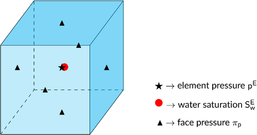
Given a porous domain partitioned into a set of nonoverlapping hexahedra, let and denote the collection of the grid elements and faces of size and , respectively. With reference to the characteristic hexahedral element of the grid depicted in Figure 1, the pressure unknowns are located on the element centroid, , and on each face barycenter, . The water saturation, , instead, is computed only on the element centroid. Let also and be the depth (positive downward) of the element centroid and faces, respectively. In the following, we describe the discretization of the PDEs in Equations (1b), (5a), and (5b).
Equation (1b) is integrated by using the approximation space for pressures ( and ) and water saturation (), while the MHFE method in the lowest-order Raviart–Thomas space49 is used to discretize the velocity (. In a 3-D setting, the latter space consists of local piecewise trilinear vector functions, , defined for each face belonging to element E. These basis functions satisfy the two properties recalled in Nardean et al..50 The unknowns and express the average value of the relevant physical quantities within the element, whereas plays a similar role for the faces. The face pressures in the MHFE method act the part of Lagrange multipliers, whose introduction is aimed at enforcing the continuity of the normal component of the fluxes across the inter-element faces.
2.2.1 The MHFE-FV system of equations
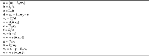
3 FULL BLOCK PRECONDITIONER
4 NUMERICAL TESTS
The computational performance of the proposed block preconditioner has been assessed in five numerical applications, including both academic and realistic settings. In the first four tests (denoted as Test 0, 1, 2, and 3), we considered a domain reproducing a planar reservoir discretized with a pair of uniform Cartesian grids referred to as coarse and fine, respectively. The coarse grid is used only in Test 0, while the fine one, displayed in Figure 2A, is considered in Tests 1 to 3. By distinction, in Test 4, the plain reservoir has been deformed into a dome formation resulting in a non-Cartesian grid built upon the fine discretization (Figure 2B). The production scenario is common to all tests and simulates a waterflooding process by means of a couple of injection and production wells located at two opposite corners. All grids have been created with Gmsh software.51

The reservoir in Test 0, discretized by the coarse grid, is characterized by homogeneous and isotropic permeability and the gravitational forces are taken into account. The main purpose of this application is to analyze the structure of and and how it typically evolves during an unsteady simulation. We compare also the eigenspectrum of the exact and inexact versions of the Schur complements to evaluate the spectral effect of the approximations.
As to Tests from 1 to 4, they are characterized by different settings for the grid type, porosity and permeability fields with gravity possibly taken into account. One of the objectives of the study is to analyze the robustness and effectiveness of the preconditioner in tackling the ill-conditioning of the systems of equations originating from models with highly heterogeneous and anisotropic permeability distributions. On the other hand, gravity modifies the overall problem structure by introducing an additional nonzero coupling block in the Jacobian. A summary of Test 0–4 settings is provided in Table 1.
| Test | 0/2 | 1 | 3 | 4 | ||
|---|---|---|---|---|---|---|
| Reservoir type | Planar | Planar | Planar | Dome | ||
| Cond. tensor properties | Homogeneous | Homogeneous | Heterogeneous | Heterogeneous | ||
| Isotropic | Isotropic | Anisotropic | Anisotropic | |||
| Cond. tensor type | Diagonal | Diagonal | Diagonal | Full | ||
| Horiz. conductivity | [m/d] | 1.E-12 | 1.E-12 | [3.53E-15, 1.97E-8] | [3.53E-15, 1.97E-8] | |
| Vert. conductivity | [m/d] | 1.E-12 | 1.E-12 | [5.92E-19, 5.92E-9] | [1.E-13, 5.92E-9] | |
| Porosity | [-] | 2.5E-1 | 2.5E-1 | [3.80E-5, 4.37E-1] | [3.80E-5, 4.37E-1] | |
| Oil spec. gravity | [kPa/m] | 8.00 | - | - | - | |
| Water spec. gravity | [kPa/m] | 9.81 | - | - | - |
- Note: The values of the permeability and porosity in brackets are the minimum and maximum of the SPE10 model portion used herein. The distribution of the relevant values in the domain follows that of the SPE10 data set. Common settings: (oil dynamic viscosity) kPa d, (water dynamic viscosity) kPa d, (rock compressibility) , (residual oil saturation) , (irreducible water saturation) , (initial water saturation) .
Test 1 is the basic benchmark with homogeneous isotropic permeability, uniform porosity and no gravity. Such a simplified setting introduces a baseline for the preconditioner and assesses the effect of the inexact application of blocks , , and on the solver performance. Test 1 is also benchmarked against global incomplete LU factorizations with variable fill-in. In Test 2, gravity is added, whereas in Test 3, a highly heterogeneous and anisotropic permeability field with abrupt spatial leaps, as retrieved from the upper layers (Tarbert formation) of the 10th comparative SPE data set,52 is introduced. The porosity distribution follows that of the SPE10 model as well. This test is aimed at evaluating the robustness and efficiency of the proposed block preconditioning framework in a real-world setting. Finally, in Test 4, the performance analysis is further stressed by considering a non-Cartesian discretization with full tensor heterogeneous and anisotropic permeability. The wells are vertical and extend through the whole reservoir thickness. The injection well operates at a constant rate, while the production well at a fixed bottom hole pressure (BHP). The fine discretization grids (both Cartesian and non-Cartesian) have 12,500 elements and 40,625 faces, for a total of 65,627 system unknowns.
GMRES,53 restarted every 200 iterations, is chosen as linear solver to address the series of linearized systems (12) stemming during the simulation. The exit criterion for the iteration count is based on the reduction of the 2-norm of the Jacobian system residual below a defined tolerance, that is, , where i is the iteration number and 1.E-6. For the nonlinear solver, instead, the termination test relies on the absolute residual check. In particular, given the different nature of the unknowns, that is, pressures and saturation, the residual is broken down accordingly and the 2-norm of the single blocks evaluated separately: , where 1.E-6.
4.1 Test 0
The objective of this preliminary test is to analyze the structure of and and its expected evolution during a typical unsteady simulation. In a waterflooding process, in fact, the number of nonzeros of evolves as a result of the water propagation in the reservoir. It is indeed the change in the water saturation that causes an increase in the density of , with a limited role played by pressure. Assuming that the reservoir is initially fully saturated of oil and water is present at its irreducible saturation, the most significant stencil enlargement is noted in blocks , , and (see also Appendix B.1), which are associated with the elemental water mass conservation equations. Knowing how the Schur complement structure evolves because of these variations is important to drive the selection of the local preconditioner.
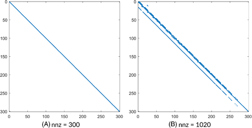
We consider the planar reservoir in Figure 2A discretized with 300 cells, with homogeneous material properties and gravity taken into account. The simulation runs for 220 days and, at the end, half domain is water saturated. Figure 3A,B shows the pattern of at the beginning and end of the simulation, respectively. From an initially diagonal structure, the stencil of is progressively enriched by a limited number of fill entries, which remain pretty clustered around the main diagonal. Such entries generate a banded nearly-lower triangular structure resembling the one typically expected in purely advective problems. This inspection suggests that a simple diagonal scaling or an incomplete factorization with no fill-in are good candidates for the application of , the former especially during the first stages of a transient simulation. Moreover, this guarantees also that the use of the diagonal in the computation of is expected to provide a good approximation of .
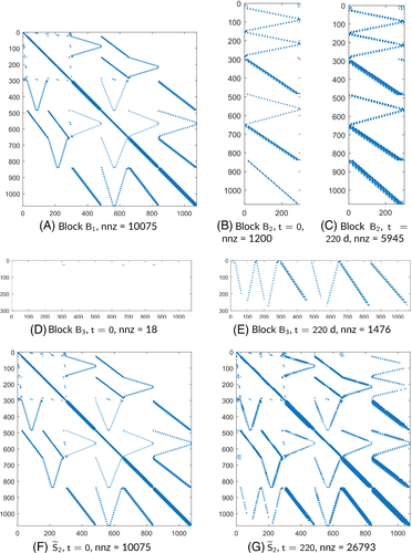
The structure of is more complicated. We can split this matrix into three contributions (see Equation (15)): , , and , with . The pattern of (Figure 4A) does not change over time and that of slightly increases (Figure 4B,C). By distinction, reflects the waterflooding evolution. It is almost empty at the beginning, with nonzeros only in the rows linked to the injection wells (Figure 4D), then it is progressively filled as the cells are flooded (Figure 4E). The evolution of block modifies the weight of the product over . At the beginning of the simulation, and . Then, the stencil enlarges as is filled and P becomes more influential. Looking at Figure 4F,G, it is also expected that both a Jacobi and a zero fill-in factorization should not be effective to approximate the application of . In this case, an incomplete factorization with fill-in, for instance, would be preferable.
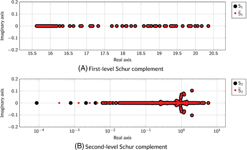
Finally, we compare the eigenspectrum of and with that of the exact Schur complements and at the end of the simulation (Figure 5). The eigenvalue distribution largely overlaps for both Schur complements, proving that the inexact computations are expected to be good approximations with no detrimental effect to the original conditioning. Notice also that the eigenvalues of are real and rather clustered away from zero.
4.2 Test 1
The simulated time interval spans 600 days of production covered in 196 time steps, whose size is dynamically adjusted during the simulation following the approach in Abushaikha et al..21 The maximum time step size is four days with the Courant–Friedrichs–Lewy (CFL) number54, 55 up to 8.56. The main model results are displayed in Figure 6 in terms of pressure, water saturation and fluid velocity. Moreover, Figure 7 shows the water front advancement from the injector toward the producer captured at some representative times along the vertical section connecting the wells. The shape of the profiles recalls that of the classical Buckley–Leverett benchmark,56 since the simulated physical process is the same and the model setting is similar.
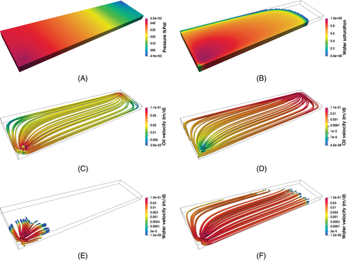
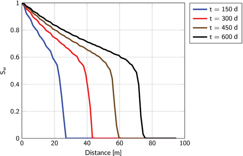
Figure 8A shows the number of iterations to converge of the first Jacobian system per time step. It can be seen that the performance stabilizes after the maximum time step size is achieved, which, in this case, occurs at the 57th step ( d). After this point, the average performance appears to be a meaningful indicator. The profiles are obtained with different approximations for , , and , as reported in Tables 2 and 3.

| # | |||||
|---|---|---|---|---|---|
| 1 | Diag | Ex | Ex | 3306 | 5.99 |
| 2 | Diag | ILU(0) | Ex | 3396 | 6.25 |
| 3 | Diag | Diag | Ex | 7490 | 15.08 |
- Note: Ex stands for exact application, which is carried out through Matlab's operator. The cumulative number of nonlinear iterations, , is 576.
| # | [s] | [s] | [s] | [s] | [s] | [s] | ||||||
|---|---|---|---|---|---|---|---|---|---|---|---|---|
| 1 | Diag | ILU(0) | 100599 | 21.09 | 1213.30 | 1234.39 | 2.617 | 180.31 | 0.04 | 2.24 | 2.28 | 2.811 |
| 2 | ILU(0) | ILU(0) | 98380 | 21.07 | 1182.86 | 1203.93 | 2.678 | 175.01 | 0.04 | 2.16 | 2.20 | 2.879 |
| 3 | Diag | ILU() | 52839 | 1877.24 | 391.81 | 2269.05 | 2.469 | 97.54 | 3.27 | 0.75 | 4.02 | 2.391 |
| 4 | ILU(0) | ILU() | 48283 | 1879.81 | 348.62 | 2228.43 | 2.533 | 85.44 | 3.26 | 0.62 | 3.89 | 2.466 |
| 5 | Diag | ILU() | 45408 | 1936.41 | 317.19 | 2253.60 | 2.932 | 83.84 | 3.37 | 0.61 | 4.98 | 2.836 |
| 6 | ILU(0) | ILU() | 41048 | 1937.03 | 280.24 | 2217.27 | 2.996 | 72.36 | 3.37 | 0.50 | 3.87 | 2.909 |
| 7 | Diag | ILU() | 29248 | 2046.91 | 210.54 | 2257.45 | 4.948 | 53.99 | 3.56 | 0.40 | 3.96 | 4.762 |
| 8 | ILU(0) | ILU() | 26220 | 2050.34 | 191.28 | 2241.62 | 5.011 | 46.09 | 3.57 | 0.34 | 3.91 | 4.834 |
- Note: For all the runs, .
- a .
- b .
- c .
As to the block preconditioner, we first analyze the effect of the inexact application of , , and on the overall performance. This investigation allows to understand where most of the efforts are needed to optimize the solver effectiveness, by identifying the blocks requiring a higher-quality local approximation. We used either diagonal scaling, or incomplete factorization, or exact application of the inverse in different combinations. In Table 2, we mainly considered the first two terms, that is, and , whereas, in Table 3, the appropriate setting for the second block is evaluated again and we focused on the approximation of . The analysis is carried out considering both the global and local (average) performance of the preconditioned linear solver.
Starting from Table 2, the outcome of run 1 tells that the diagonal approximation for is appropriate for this block. Replacing the application with an ILU(0), as in run 2, leads to a marginal increase in the total number of linear iterations (2.7%). By distinction, a diagonal approximation of causes a 120.6% increase in the global iteration count. Therefore, a more detailed comparison is needed by taking into account the computational effort to compute and apply the preconditioner. In any case, the outcome of this analysis suggests that the overall solver performance mainly relies on the quality of the approximation for , as expected from the preliminary analysis carried out on Test 0. This is investigated in Table 3. Here, two incomplete factorization variants, that is, ILU(0) and threshold-based ILU(), have been tested for . The tests have been carried out for both the diagonal scaling and ILU(0) factorization of . The results show that, although ILU() can significantly reduce the cumulative linear iteration count, , and solving time, , this strategy typically does not pay off because of the higher set-up cost, . We also observe that the difference between diagonal scaling and ILU(0) factorization for is not as significant in terms of total time. Nevertheless, the latter appears to be more effective, hence it is chosen as default option in the next tests. Furthermore, the effect on the preconditioner density, and , is almost negligible.
The analysis in Section 4.1 highlighted that tends to become denser as the simulation proceeds. This result is confirmed by the outcome of Table 3, which shows that the preconditioner density is likely to increase slowly but steadily during the simulation when ILU(0) is used for , whereas the opposite trend is noted with ILU(). Specifically, compare the density values in the columns and (runs 1,2 vs. 3–8). In any case, filtration techniques can be applied to sparsify and stabilize the memory occupation, if necessary. Of course, the application of such techniques can affect the set-up cost.
The performance of the block preconditioner is also benchmarked against that of global incomplete LU factorizations with no or variable fill-in. The ILU decomposition is built upon the Jacobian matrix preliminary reordered by means of the reverse Cuthill–McKee algorithm.26 The outcome is provided in Table 4. While with ILU(0) GMRES does not converge within 1000 iterations in most of the linearized systems, threshold-based ILU delivers better results but at a significant higher computational time with respect to our block preconditioner, where the greatest share is due to the set-up cost (compare, in this regard, columns , , , and in Tables 3 and 4). Notice also that reducing the threshold value, , below 0.01 results in a degradation of the preconditioned solver performance, most likely caused by the introduction of detrimental near-zero entries in the triangular factors.
| Type | [s] | [s] | [s] | [s] | [s] | [s] | ||||
|---|---|---|---|---|---|---|---|---|---|---|
| ILU(0) | NC | - | - | - | 1.173 | - | - | - | - | 1.165 |
| ILU() | 107022 | 4716.76 | 1400.90 | 6117.65 | 1.608 | 199.4 | 8.15 | 2.73 | 10.88 | 1.568 |
| ILU() | 68425 | 4675.91 | 682.88 | 5358.79 | 2.494 | 134.65 | 8.09 | 1.45 | 9.54 | 2.512 |
| ILU() | 78911 | 4796.63 | 1028.53 | 5825.16 | 3.872 | 158.19 | 8.33 | 2.27 | 10.60 | 4.330 |
- a .
- b .
- c .
4.3 Test 2
In this test, gravity is taken into account to evaluate its impact on the solver performance, whereas the production scenario and the other model settings are the same as in Test 1. The simulated time interval spans 250 days, with a maximum time step size of 0.5 days. This value is lower with respect to the previous test and it was set to keep the number of nonlinear iterations below 6–7. The simulation takes 526 time steps to conclude, with the maximum size achieved at the 37th step ( d) and the CFL number up to 2.26. Figure 9A shows the water saturation field at the end of the simulation on the whole domain, while Figures 9B–D report the solution along a vertical section through the wells. The injected water propagates through the reservoir toward the producer, and simultaneously tends to accumulate at the bottom due to the action of gravity.
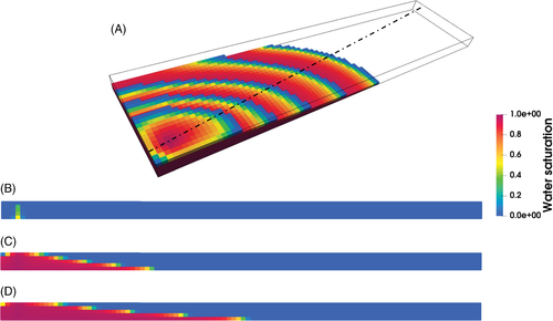
Table 5 reports the main results of the preconditioner performance analysis, which can be compared with those in Table 3. Based on the cumulative number of nonlinear iterations and the smaller time interval simulated than in Test 1, we can say that the problem is more challenging for the outer nonlinear solver, but the effect of gravity on the performance of the preconditioned linear solver appears to be negligible. The number of linear iterations, , in fact, along with the density, , are similar to those in Test 1. This result is consistent with the observations in Section 4.1. The extra nonzero block appearing with gravity, , is required only in the computation of the product P for (specifically in ). We observed also that the importance of the P term is not constant during a simulation, but evolves depending on the water distribution within the reservoir. Even in this application, the threshold-based incomplete factorization, though succeeding in deflating the iteration count significantly (runs 2–4), does not outperform ILU(0) in terms of CPU time. A similar behavior of the preconditioner density, which grows during the simulation when an ILU(0) approximation is used, can be noted as well.
| # | [s] | [s] | [s] | [s] | [s] | [s] | |||||
|---|---|---|---|---|---|---|---|---|---|---|---|
| 1 | ILU(0) | 528006 | 118.12 | 6215.87 | 6333.99 | 2.531 | 153.24 | 0.04 | 1.74 | 1.78 | 2.569 |
| 2 | ILU() | 257633 | 10723.27 | 1813.43 | 12536.71 | 2.395 | 74.89 | 3.27 | 0.51 | 3.78 | 2.385 |
| 3 | ILU() | 214446 | 11041.27 | 1428.21 | 12469.48 | 2.808 | 62.23 | 3.37 | 0.40 | 3.77 | 2.794 |
| 4 | ILU() | 132703 | 11626.79 | 939.03 | 12565.82 | 4.618 | 38.74 | 3.54 | 0.27 | 3.81 | 4.590 |
- Note: For all the runs, .
- a .
- b .
- c .
4.4 Test 3
The homogeneous isotropic permeability field of Test 1 and 2 is here replaced by a highly heterogeneous and anisotropic distribution retrieved from the SPE10 data set (see Figure 10A,B). Notice the wide range of values, spanning approximately ten orders of magnitude, and the abrupt discontinuities, especially in the vertical permeability (Figure 10B), which make this test numerically challenging. The porosity distribution, displayed in Figure 10C, follows that of the SPE10 model as well. Given the similar performance of the linear solver with and without gravity and the greater computational burden for the outer nonlinear solver observed in Test 2, in this application we decided to neglect the gravitational effects. The simulation runs for 250 days with a maximum time step size of 1.5 days, achieved at the 42nd step ( d), and a total number of 198 steps. The CFL value is up to 30.27. At the end of the simulation, large portions of the oil in the reservoir have been displaced by water and breakthrough occurs at the producer. Figure 11 provides some model insights in terms of water saturation at d and d.
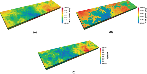

Table 6 summarizes the results obtained for different approximations of . For two of them, the number of iterations to solve the first linearized systems vs. time step is displayed in Figure 8B. Although the permeability distribution is highly heterogeneous and anisotropic, the number of iterations approximately stabilizes after the maximum time step size has been achieved like in Test 1 (see also Figure 8A). By comparing the iteration counts, and , of run 1 with the counterpart in Table 3, we can appreciate the effect of the ill-conditioning caused by the extremely wide range of permeability and, with a minor role, porosity values. We carried out a sensitivity analysis on the threshold value for ILU() (runs 2-4), which appears now to pay off with respect to the zero-fill incomplete factorization (run 1). Despite the higher set-up cost, the cumulative total solving time, , reduces as the threshold is decreased, while the density growth is firmly under control. Moreover, the cumulative number of linear iterations is reduced by 2.6 to 6.5 times. The sensitivity analysis shows that a threshold value for the drop tolerance in the range between 0.001 and 0.005 appears to be a good trade-off between fast convergence and the need of restraining the memory occupation.
| # | [s] | [s] | [s] | [s] | [s] | [s] | |||||
|---|---|---|---|---|---|---|---|---|---|---|---|
| 1 | ILU(0) | 227024 | 25.10 | 3010.35 | 3035.45 | 2.789 | 395.61 | 0.05 | 5.35 | 5.40 | 2.952 |
| 2 | ILU() | 87747 | 2097.04 | 925.42 | 3022.46 | 1.994 | 148.68 | 3.40 | 1.61 | 5.01 | 1.962 |
| 3 | ILU() | 68016 | 2089.94 | 612.96 | 2702.90 | 2.224 | 115.11 | 3.39 | 1.07 | 4.56 | 2.186 |
| 4 | ILU() | 35107 | 2179.04 | 240.48 | 2419.53 | 3.156 | 58.78 | 3.53 | 0.41 | 3.94 | 3.095 |
- Note: For all the runs, .
- a .
- b .
- c .
4.5 Test 4
Modeling the fluid flow with a high approximation accuracy in non-Cartesian grids using full tensor permeability properties is an important requirement for modern simulators. This is also a challenge for most discretization schemes, which is effectively addressed by the MHFE method.21 In the last test case, a dome reservoir is taken into consideration with this challenging setting. Porosity and permeability are again taken from the SPE10 data set with the horizontal/vertical anisotropy ratio up to 1.E5. The full permeability tensor is obtained from the original diagonal tensor by rotating the local element axes so as to follow the curvature of the dome formation, similarly as in Nardean et al..50 The main effect of non-Cartesian grid and full tensor permeability on the model can be seen in the stencil of block , which is enlarged with respect to the previous setting. This is because the local matrices , which are block diagonal with a diagonal permeability tensor and a Cartesian grid, become full (see Equation (8)). Therefore, while in the former setting there are up to three nonzero entries in each row of , such limit increases to eleven in the latter. On the contrary, the stencil of the other blocks in the Jacobian is not affected by the change in the grid or permeability tensor type. Figure 12 shows some model insight in terms of water saturation distribution, while the computational performance of the linear solver is summarized in Table 7. As in Test 3, the threshold-based incomplete factorization performs better than the no-fill variant in terms of CPU time. The sensitivity analysis on the threshold shows that a value between 0.0005 and 0.001 can be a good compromise in terms of memory footprint and computational efficiency, which is a little lower than in Test 3. Notice also that the density of the preconditioner in this test is lower than in Test 3 when the same value for is used in the incomplete factorization.

| # | [s] | [s] | [s] | [s] | [s] | [s] | |||||
|---|---|---|---|---|---|---|---|---|---|---|---|
| 1 | ILU(0) | 278513 | 28.61 | 4395.75 | 4424.36 | 1.647 | 489.99 | 0.05 | 7.88 | 7.93 | 1.777 |
| 2 | ILU() | 234091 | 2162.13 | 3672.03 | 5834.16 | 1.411 | 433.84 | 3.53 | 6.92 | 10.45 | 1.405 |
| 3 | ILU() | 70266 | 2220.04 | 854.30 | 3074.34 | 2.235 | 119.86 | 3.63 | 1.50 | 5.13 | 2.217 |
| 4 | ILU() | 54840 | 2271.59 | 640.49 | 2912.08 | 2.802 | 93.55 | 3.71 | 1.12 | 4.83 | 2.778 |
| 5 | ILU() | 28902 | 2390.80 | 370.26 | 2761.06 | 4.807 | 49.48 | 3.91 | 0.64 | 4.55 | 4.762 |
- Note: For all the runs, .
- a .
- b .
- c .
- d .
5 DISCUSSION AND CONCLUSIONS
The accurate and efficient numerical modeling of two-phase flow in porous media is a key tool for petroleum engineering applications. In our formulation of the mathematical problem, the demand for higher accuracy of the solution is met by means of a MHFE discretization of Darcy's law, whereas the coupled nonlinear system is addressed in a fully implicit unconditionally stable way by a Krylov solver. Such an approach requires the solution to a sequence of nonsymmetric large-size and often ill-conditioned linearized systems of equations with the Jacobian matrix. This is the most time and resource consuming task in a simulation. Supplying a proper preconditioner to the Krylov subspace solver is decisive to damp such cost and make the fully implicit approach attractive with respect to sequential techniques.
- a diagonal preconditioner for and an ILU(0) factorization for proved to be cheap and appropriate choices. Finding an approximation to apply , conversely, requires a little more care, since it is the factor that mostly governs the effectiveness of the block preconditioner;
- depending on the problem features, different strategies can be followed for . In general, for simple settings with homogeneous isotropic permeability, ILU(0) is already a good approximation, whereas in case of heterogeneous materials it is necessary to move to higher-quality variants, such as the threshold-based ILU();
- accounting for gravity in the simulation does not seem to affect the linear solver performance much, while it can increase significantly the computational burden of the nonlinear solver;
- when fill-in is allowed in the incomplete factorization of the second-level Schur complement, the preconditioner density is under control during the simulation and it remains approximately constant. Conversely, a slight, but steady, growth is observed with the ILU(0) version, consistently with the progressive increase of number of water flooded cells;
- in all cases, the proposed solver is stable and robust, being able to provide the solution under any condition achieved during the full-transient simulation and with strongly heterogeneous and anisotropic material properties, with no increase of the average computational cost required by the linear solver.
Ongoing research focuses on applying efficient sparsification techniques to and have a full control of the memory occupation. Since the set-up cost increases as a result of this additional operation, filtration can be performed only once a certain memory limit has been exceeded. Additional tests are underway to extend the preconditioning framework to a fully parallel environment, by carrying out appropriate scalability tests and experimenting the introduction of multigrid and/or multiscale approaches as local approximations of and .
ACKNOWLEDGMENT
This publication was supported by the National Priorities Research Program grant NPRP10-0208-170407 from Qatar National Research Fund.
Author Contributions
Stefano Nardean: Conceptualization, software, writing–original draft. Massimiliano Ferronato: Methodology, supervision, writing–review & editing. Ahmad S. Abushaikha: Funding acquisition, supervision, writing–review & editing.
Conflict of Interest
The authors declare no potential conflict of interests.
APPENDIX A.
A.1 Peaceman well model
APPENDIX B.
B.1 Jacobian blocks' structure
Biographies

Stefano Nardean is PhD candidate in Sustainable Energy at Hamad Bin Khalifa University. The focus of his research is the development of efficient linear solvers for reservoir simulations applications. Other scientific interests, within the subject of applied numerical analysis, concern the modeling of deformation and flow processes in porous media, with specific applications in the field of subsurface hydrology and petroleum engineering.

Massimiliano Ferronato is Professor of Numerical Analysis at the University of Padova, Italy. He has authored and co-authored about 170 papers in international journals and conference proceedings. The main scientific interests concern the design of numerical models for the solution of PDEs governing coupled processes in porous media along with the analysis, development and implementation of block preconditioners for saddle-point problems arising in geoscience applications.

Ahmad Abushaikha is Associate Professor at Division of Sustainable Development at Hamad Bin Khalifa University. He has authored and co-authored about 45 research publications in international journals and conference proceedings. His research interests are in reservoir simulation, fluid flow in porous media, discretization schemes, high performance computing, petroleum engineering and enhanced recovery mechanisms.


