A qualitative analysis of a Mycoplasma genitalium epidemiological model
Abstract
The objective of the article is to present a qualitative analysis of a mathematical model for the spread of a sexually transmitted infection caused by Mycoplasma genitalium. Recent investigations revealed that this pathogen is becoming resistant to the use of macrolides and can turn into a superbug in the next few years. We present an epidemiological model to describe the spread of the disease. The equilibrium points are computed, and their local and global stability are studied. In order to make the mathematical problem more realistic, we propose two different optimal control problems that establish a balance between the number of infected individuals and the use of macrolides. Several numerical illustrations regarding the solutions of the proposed problems will be provided.
1 INTRODUCTION
In July 2018, the British Association for Sexual Health and HIV came up with a concern that the little known but common sexually transmitted infection (STI) called Mycoplasma genitalium (M. genitalium) could become a “superbug” within 10 years. In most cases, infections caused by the pathogen M. genitalium have no symptoms and when they have, they can be mistaken with other STI, such as chlamydia or gonorrhea. This in turn can lead to prescriptions of wrong antibiotics, inappropriate dose or inadequate time of treatment, which can result in an emerging increase of in antimicrobial resistance and, consequently, a global public health problem.
The first cases of M. genitalium have been identified in 1981 in two men with nongonococcal urethritis.1, 3 During a long time it was not a cause of concern mainly because it was not associated with serious illness or sequelae. For a period, it was even discussed whether treatment would be necessary when this bacterium was found, since in the vast majority of cases it appeared as an asymptomatic infection.2 However, in the last decade, several studies associated the infection by M. genitalium to acute and chronic urethritis in men and vaginal discharge, cervicitis and pelvic inflammatory disease in women. Additionally, it can cause serious risks of endometriosis, spontaneous abortion, premature birth, and infertility. According to community based studies from the United States, United Kingdom, Australia, and Scandinavia, the estimated prevalence of M. genitalium is in the range 1%–3% in men and women population (see Reference 3 and references therein).
M. genitalium is the smallest known bacterium that can replicate itself. In a laboratory setting, this fastidious bacterium is extremely slow growing and therefore culture is not appropriate for diagnosis.4 Nucleic acid amplification tests (NAATs) are the only useful diagnostic method that detect M. genitalium DNA or RNA in clinical specimens.5 NAATs use polymerase chain reactions that can be performed on multiple sample types, including urethral, vaginal, and cervical swabs, first void urine, and endometrial biopsies. One of the main obstacles for diagnosing the M. genitalium is the lack of commercially available diagnostic tests. NAATs for diagnosing M. genitalium use assays that were developed for the research setting and, as a result, NAATs are only available in reference labs, usually at large university hospitals. Also these methods of diagnosis are extremely expensive. Nevertheless, it is also recommended that, where possible, all positive M. genitalium should be tested for macrolide resistance mediating mutations.6
Usually, the first line treatment is done with a single 1g oral dose of the macrolide azithromycin. However, mutations in region V of the 23S ribosomal RNA gene are becoming frequent, thus inducing a powerful strain of the bacterium resistant to macrolides.7 Owing to emergence of resistance, the efficacy of azithromycin has drastically decreased during the past decade, thus requiring more aggressive treatments.5 This represents a big problem for health authorities, since this mutation can lead to a dominant strain of the bacterium resistant to antibiotics. This is where mathematical modeling comes into play.
Mathematical modeling is an essential tool in studying a diverse range of infectious diseases that have impact, not only in terms of physical or mental suffering, but also on the social and economic level. Main goals include the study of disease spread, the better understanding of transmission mechanisms and those properties who are most influential in the spread, and also in the practice of disease management and control.8 In the latter, mathematical models play an important role in making public health decisions on the control of infectious diseases.9
The importance of modeling infectious diseases dates back to 1760, when Daniel Bernoulli came up with a solution to his mathematical model on smallpox. However, only in the 20th century, mathematical methods have been recognized as fundamental tools in epidemiology.10 Since then, a huge variety of models has been formulated, mathematically analyzed and applied to infectious diseases, what can be checked in several reviews of the literature (see, for instance, References 8, 9, 11).
Following this reasoning, a mathematical model to investigate the contribution of the de novo macrolide resistance mutations to the spread of the antimicrobial resistant M. genitalium has been proposed in Reference 12. It consists on the SIS (SusceptibleInfectiousSusceptible) model, since an infection by M. genitalium does not confer immunity. Thus, susceptibles become infected and then become susceptible again upon recovery. The model has been fitted to data from France, Sweden, and Denmark and the authors observed that the high probability of the de novo macrolide resistance mutations accelerates the spread of antimicrobial resistant M. genitalium.
In this article, a qualitative analysis of the M. genitalium epidemiological model proposed in Reference 12 is presented. Namely, we study the existence and uniqueness of solutions of the proposed system of ordinary differential equations, determine the equilibrium points of the system, and finally study their global stability. Moreover, two optimal control problems will be formulated in order to give strategies to control the spread of the de novo macrolide resistance mutations due to the emergence of azithromycin resistant M. genitalium.
The organization of the article is the following. In Section 2, we recall the SIS mathematical model proposed in Reference 12, and prove the existence and uniqueness of solutions in Section 3. In Section 4, we determine the two equilibrium points of the system, namely the disease free equilibrium point and the endemic equilibrium point, and study their stability. In Section 5, we improve the mathematical model given in Reference 12 by allowing the treatment rate to vary along time, with the formulation of two different optimal control problems. Necessary optimality conditions are derived using the Pontryagin maximum principle. For these problems, a trade-off between the spread of the infectious individuals and the administration of macrolides is established. This in turn will be helpful for health organizations to make decisions regarding the control of the spread of resistant strains of M. genitalium. Several numerical illustrations will be provided in Section 6 for the two optimal control problems, in order to corroborate the theoretical issues derived along the sequel. Finally, using real data provided by the Public Health England, we estimate the transmission and treatment rates to study the spread of M. genitalium in England as a study case in Section 7. We finish the article with some epidemiological implications.
2 MYCOPLASMA GENITALIUM EPIDEMIOLOGICAL MODEL
- s, the susceptibles, that is, individuals that can become infected if exposed to the bacterium;
- , individuals infected with a drug-susceptible strain of the bacterium;
- , individuals infected with a drug-resistant strain of the bacterium.
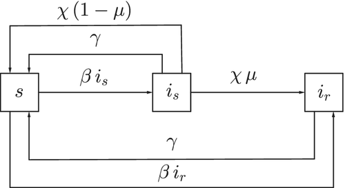
| Disease transmission rate | |
| Natural rate of recovery from both infections (without treatment) | |
| Treatment rate of infected individuals | |
| Probability of gene mutation causing resistance to the antibiotic during treatment |
3 EXISTENCE OF NON-NEGATIVE SOLUTIONS
First, we prove that the problem is well-posed.
Proof.System (1) can be written in the form , where for ,
Now we prove the non-negativity of the solution for system (1) and (2).
4 EQUILIBRIUM POINTS AND STABILITY
- a disease free equilibrium point , and
- an endemic equilibrium point , if .
Theorem 3.The disease free equilibrium point is
- 1.
locally asymptotically stable if ;
- 2.
unstable if ;
If , then a critical case occurs.
Proof.The Jacobian matrix (5), evaluated at the disease free equilibrium point, is the following:
Since the spectrum of matrix (6) is
Theorem 4.If , then model (1) has an endemic equilibrium point given by , and is locally asymptotically stable.
Proof.In this case, the Jacobian matrix is given by
In the field of epidemic models, one of the most challenging questions is the stability analysis.15-20
Theorem 5.If , then the disease free equilibrium point of model (1) is globally asymptotically stable.
Proof.Consider the following Lyapunov function Differentiating V with respect to time gives
Thus, for all . Moreover, if and only if . Consequently, by LaSalle's Invariance Principle,21 the disease free equilibrium point is globally asymptotically stable.
Theorem 6.Let . Then, the endemic equilibrium point of model (1) is globally asymptotically stable.
Proof.Consider the following Lyapunov function
Observe that, for all , . In fact, if , and since , we get that
- , the basic reproduction number is and so the disease free equilibrium point is globally asymptotically stable;
- , and so the endemic equilibrium point is globally asymptotically stable;
- , and so the endemic equilibrium point is globally asymptotically stable.

In Figure 3 we present the evolution of the bacterium propagation, taking into consideration different values of the total number of infected individuals at the initial time, as well as different values of the transmission rate .
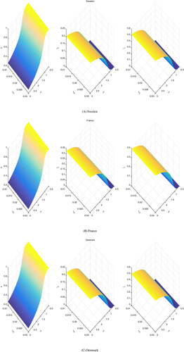
Note that all the sensitivity surfaces are drawn at time years, at which none of the populations has reached a steady state, the dynamics is still changing in time. But they are comparable, as all of them are drawn at this time.
All the figures show that the influence of the initial condition on the total number of infected does not influence the outcome as it is expected, due to the global stability of the equilibrium points.
Instead, the contact rate has a relevant role in the disease propagation. A steady increase of the infected is observed with an increasing value of this rate. In each country, the attained size of the infected individuals, for the maximum explored value of the transmission rate, differs. For France, the fraction of infected with a drug-susceptible strain of the bacterium lies between 0.30 and 0.35, probably attaining the value 0.32 while the corresponding fraction of infected with a drug-resistant strain attains the value 0.4. In Sweden, the former is only 0.2 while the drug-resistants are a half of the total population, thereby the situation would be worse than in France. The situation in Denmark appears to be a little better than in Sweden, as the drug-susceptibles are slightly above the value 0.2, maybe around 0.22, at the expense of the drug-resistants that fall slightly below 0.5.
The bottom line is that the drug-resistants in all cases are bound to increase to an alarming percentage of the population under scrutiny.
5 AN OPTIMAL CONTROL APPROACH
So far, we considered a constant rate of infected individuals that will receive treatment during the process, . Since treatment involves costs, and in any situation, health organizations have to find a balance between financial issues and diseases control. In this section we consider a treatment rate depending on time, , which will be the control. We assume that the control is bounded, , in order to deal with a more realistic model and two distinct optimal control problems will be proposed.
Parameters , , and are positive real constants that can be interpreted as weights associated to the infected individuals and to the treatment rate, respectively. These weights will provide a scaling for the magnitudes of the quantities . For the sake of simplicity we fix . The goal is to minimize the number of infected individuals and and at the same time the treatment rate .
Theorem 7. ([24])There exists an optimal control and a set of corresponding solutions that minimize the objective functional (7) subject to (8) and (9). Moreover, there exists an adjoint function ,, such that is a solution of the following equations:
- 1.
The control system
that is, system (8); - 2.
The adjoint system:
() - 3.
The transversality condition
()
Furthermore, the following minimization condition is fulfilled:
Proof.The existence of an optimal control is an immediate consequence of Reference 25 (corollary 4.1). In fact, it follows due to:
- the convexity of integrand of with respect to the control ;
- a priori boundedness of the state solutions;
- the state system (8) satisfies the Lipschitz property with respect to the state variables since state solutions are bounded.
The deduction of the necessary optimality conditions is a standard result from the Pontryagin's minimum principle. If is an optimal control, there exists a nontrivial mapping , such that the following equations are satisfied for :
- The control system
- The adjoint system:
- the transversality condition ;
and also the minimization condition:
Based on the priori boundedness of the state and adjoint functions and the resulting Lipschitz structure of the ODEs, we can ensure a unique optimal control for a small value of T. The uniqueness of the optimal control follows from the uniqueness of the optimality system, given by the control system (8) and the adjoint system (10), together with the transversality condition (11) and with characterization (12).
In this case, the goal is to minimize the number of infected individuals only at the final time and at the same time minimizing the treatment rate during the entire process.
The two optimal control problems are solved using a Matlab code based on Forward-Backward Sweep Method.26 The system of ordinary differential equations is solved numerically using a fourth order Runge–Kutta method.
6 NUMERICAL SIMULATIONS
Numerical simulations are shown in Figures 4 and 5 for both optimal control problems, where two values of the parameter are tested: and . The remaining parameters are and . The values of the weights and the initial conditions are , and , respectively. The corresponding dynamics are evaluated for years.
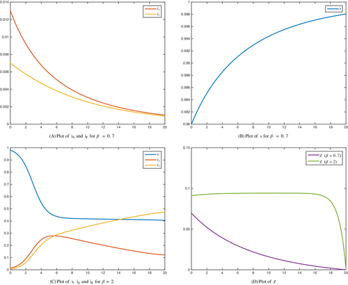
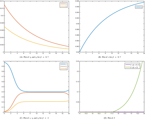
According to the values of the parameters that we fixed previously, a comparison between the performance of the two optimal control problems is shown in Table 2 for different values of .
| 0.5 | 2.7935e-5 | 1.7204e-5 | 0.0402 | 0.0232 | 9.6752e-4 | |
| 3.1170e-5 | 1.6795e-5 | 0.0425 | 0.0229 | 7.4323e-9 | ||
| 0.7 | 0.0010 | 9.2380e-4 | 0.0838 | 0.0602 | 0.0082 | |
| 0.0015 | 8.5032e-4 | 0.1052 | 0.0572 | 1.6815e-5 | ||
| 0.9 | 0.0125 | 0.0355 | 0.2154 | 0.3797 | 0.0703 | |
| 0.0326 | 0.0274 | 0.4655 | 0.3168 | 0.0037 | ||
| 1.0 | 0.0251 | 0.1170 | 0.3670 | 0.9924 | 0.1130 | |
| 0.0796 | 0.0727 | 1.0364 | 0.7009 | 0.0080 | ||
| 1.2 | 0.0501 | 0.2713 | 0.9945 | 2.7739 | 0.1212 | |
| 0.1685 | 0.1325 | 2.7244 | 1.5413 | 0.0134 | ||
| 1.5 | 0.0809 | 0.3797 | 2.1466 | 4.6418 | 0.1028 | |
| 0.2469 | 0.1832 | 4.6403 | 2.5509 | 0.0164 | ||
| 2.0 | 0.1231 | 0.4724 | 3.6664 | 6.3128 | 0.0821 | |
| 0.3313 | 0.2309 | 6.6560 | 3.6171 | 0.0173 |
As it can be observed, the optimal control problem () seems to be a better strategy to implement even for high rate of the bacterium spread. Indeed, the treatment rate on the whole time horizon for problem () is considerably lower than the treatment rate for problem (). Also, for small values of , there are no substancial differences between the number of infected individuals and at the final time T for the two problems. In both situations, independently of using problems () or (), the total number of infected individuals at the final time, , is similar. However, the number of drug-susceptible individuals either at the final time or along the time horizon is always lower with method (). The reverse situation occurs when we consider the number of drug-resistant individuals.
With respect to the administration of treatment, it can be noticed in Figures 3 and 4, that for , when we consider procedure (), the treatment rate is almost constant during the whole process except near the final time, where it decreases and vanishes. On the contrary, in problem (), the treatment rate is close to zero, except near the final time, where the treatment rate increases considerably. This is the reason why the number of infections by the drug-resistant bacterium increases and overtakes the number of infections by the drug-susceptible bacterium when we apply the treatment given by (). With the second approach, since the treatment is applied mostly near the final time, the number of infections by drug-resistant bacterium is always lower than the number of infections by drug-susceptible bacterium, even though near the final time is increasing as a consequence of the treatment increment.
Overall, the technique given by problem () seems to be more efficient since it involves less financial costs and a lower number of individuals infected by the drug-resistant strain of M. genitalium. This can be helpful for health organizations to outline a strategy to control the propagation of macrolide resistant mutations.
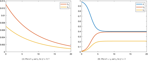
Remark 1.Although at the endemic equilibrium, and the equilibrium is globally stable, we can not ignore the class in the optimal control model, since in this case the results will be different. For example, using the same data as the ones used in Figure 4, but considering , the results are displayed in Figure 6. As it can be seen, the evolution of infected individuals is distinct when .
7 A CASE STUDY: THE SPREAD OF M. GENITALIUM IN ENGLAND
In this section we study the spread of the disease in England, using real data. In Table 3, the number of M. genitalium diagnoses per month in England is displayed. These data were provided by the Public Health England (PHE), from GUMCAD STI Surveillance System. We remark that data represent the number of diagnoses reported, and not the number of people diagnosed. Also, only a small number of sexual health services were reporting M. genitalium diagnosis codes (35 in 2016 and 67 in 2017).
| 1 | 2 | 3 | 4 | 5 | 6 | 7 | 8 | 9 | 10 | 11 | 12 | Total | |
|---|---|---|---|---|---|---|---|---|---|---|---|---|---|
| 2016 | 14 | 14 | 19 | 15 | 15 | 19 | 16 | 14 | 24 | 18 | 18 | 19 | 205 |
| 2017 | 13 | 30 | 18 | 21 | 40 | 37 | 44 | 40 | 53 | 38 | 54 | 37 | 425 |
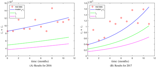
As it can be observed, the number of cases diagnosed is much lower than the number of persons infected by the bacterium. This is due to two factors. First, sometimes the disease is asymptomatic. On the other hand, since the means of diagnosis are extremely expensive, the patient may have the symptoms but a general antibiotic treatment, not specific for M. genitalium, is applied. To overcome this problem when we model the problem, and the number of total population is required, the following procedure is adopted. In the case of England, previous studies suggest that of the population is infected by this bacterium (MG prevalence is in men and in women22). So, for the population size, we take , where Total denotes the total number of cases diagnosed each year. For initial conditions, we consider the number of patients diagnosed in the first month, distributed as follows: is in class and the remaining in class .
| Error | |||
|---|---|---|---|
| 2016 | 1.186471467465153 | 0.000161634124816 | 2.810869290229194e-07 |
| 2017 | 2.409736648752084 | 0.002209748965879 | 1.398194788165466e-06 |
Based on this data, we observe that the transmission rate has increased from 2016 to 2017. Also, the strain ofM. genitalium that is resistant to treatment is increasing, which represents a serious problem to deal with for the health organizations.
In Figure 8 we present an analysis of the evolution of the disease, considering different values of the treatment rate and the disease transmission rate .
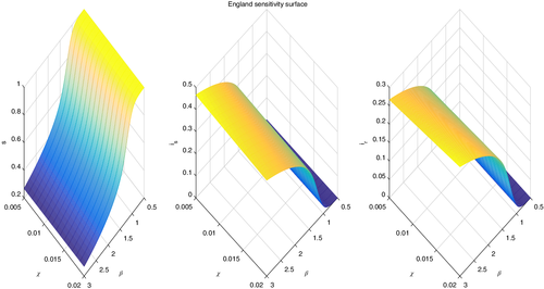
For England the situation is similar to the other countries. In this case it is the parameter that does not seem to have any substantial influence on the simulation outcome. As for , the final population fractions values for settle respectively to , , and , a situation close, but seemingly slightly better, than Sweden.
8 EPIDEMIOLOGY IMPLICATIONS
In this article, a mathematical model that simulates the spread of the drug-resistant M. genitalium within a population was studied. Equilibrium points and their stability were analyzed. Moreover, two optimal control problems have been proposed where the treatment rate is assumed to vary along the time. In one of them, besides minimizing the treatment rate, our interest was also to minimize the number of infected individuals during a certain period of time. In the other one, the objective was to minimize the number of infected individuals only at the final time. Several numerical tests have been performed in order to analyze the trade-off between the number of drug-resistant and drug-susceptible infected individuals by M. genitalium and the administration of treatment. In all the situations, the proposed mathematical model is coherent with the clinical practice since the introduction of azithromycin will considerably increase the number of drug-resistant bacterium.
An important issue that must be studied is the evolution of the disease over a long period of time. In Figure 9 we present the results obtained.
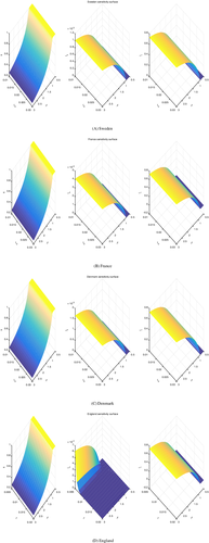
The shape of the surfaces qualitatively is the same in all cases. However, at steady state we observe the vanishing of the infected that are susceptible to drugs, while the populations are partitioned only among uninfected and infected but drug-resistant. The proportions are about of infected (drug-resistant) for all the countries, leaving only of the population uninfected. This makes sense, as these quantities are related to the infection. The only difference is the speed at which this steady state is reached, as it depends more on the present conditions in the respective countries, as well as being related to the various populations behaviors, which may differ from country to country.
ACKNOWLEDGMENTS
R. Almeida is supported by funds through CIDMA-Center for Research and Development in Mathematics and Applications, and Fundação para a Ciência e a Tecnologia (FCT), within project UIDB/04106/2020. M.T.T. Monteiro is supported by FCT—Fundação para a Ciência e a Tecnologia, within the Project Scope: UIDB/00319/2020. L. Machado acknowledges Fundação para a Ciência e a Tecnologia (FCT) for the financial support to the project UIDB/00048/2020.
CONFLICT OF INTEREST
The authors declare no potential conflict of interests.
Biographies

Ricardo Almeida received his Bachelor and Master degrees in Mathematics from University of Oporto, Portugal, and Ph.D. degree in Mathematics from University of Aveiro, Portugal. He is currently Assistant Professor in the University of Aveiro. His research interests include fractional calculus, calculus of variations, and optimal control theory. He has published 5 books and more than 80 papers in international journals.

M. Teresa T. Monteiro received the BS, MS, and Ph.D. degrees in Systems and Informatics Engineering (1990), Computational Mathematics (1996), Nonlinear Optimization (2001), respectively, from University of Minho, Portugal. She is researcher in Centre ALGORITMI, University of Minho, Portugal. She started working at the Systems and Production Department, from Engineering School, University of Minho since 1992, being assistant professor. Her research interests are multidisciplinary: optimal control and nonlinear optimization applied to epidemiological models; applications of optimization; numerical methods; mathematical modeling.

Ezio Venturino received his Ph.D. degree in Applied Mathematics from SUNY at Stony Brook in 1984. He is currently professor of Mathematics at the Dipartimento di Matematica, University of Torino, Italy. He has visited several international institutions worldwide has a wide scientific collaboration network. His research earlier focused on numerical analysis, mainly methods for integral equations, and currently on nonlinear models for biological and ecological applications.

Luís Machado received the BS, MS, and Ph.D. degrees in Mathematics from the University of Coimbra, Portugal, in 1996, 1999, and 2006, respectively. Since 1996 he has been with the Department of Mathematics, University of Trás-os-Montes e Alto Douro, Vila Real, Portugal, where he is currently an assistant professor. He is also a researcher at the Institute of Systems and Robotics—University of Coimbra, Portugal. His research interests are multidisciplinary and include optimization problems on manifolds, calculus of variations and optimal control problems.


