Computation of the reverse generalized Bessel polynomials and their zeros

1 INTRODUCTION

It is well known that generalized and reverse generalized Bessel polynomials have applications in different areas of science and technology, including applied mathematics, mathematical physics, and electrical engineering; see, for example, References 1, 2. It is interesting to mention that the reverse Bessel polynomials (a particular case of the reverse generalized polynomials) are important in filter design.³ In particular, the poles of the transfer function of a Bessel filter are basically the zeros of reverse Bessel polynomials.

Some properties satisfied by these polynomials can be found, for example, in Reference 4. For computing the polynomials, we consider the use of asymptotic expansions in terms of elementary functions given in Reference 5 and a three-term recurrence relation satisfied by the polynomials. The expansions were obtained by using the well-known Liouville-Green theory for ordinary differential equations in the complex plane.

On the other hand, several papers can be found in the literature on the approximation and study of the distribution of the zeros of generalized Bessel and reverse generalized Bessel polynomials; see, for example, References 6, 7. In this article we discuss the numerical performance of an algorithm to compute the zeros of reverse generalized Bessel polynomials ${\theta }_n(z;a)$. For this, we use the method given in Reference 8, which is based on a qualitative analysis of the approximate Liouville-Green Stokes lines and anti-Stokes lines of the differential equation satisfied by the polynomials, combined with the application of a high-order fixed-point method and carefully selected step functions. As we will see, a method to compute the polynomials ${\theta }_n(z;a)$ will be needed for evaluating the zeros. Therefore, the numerical evaluation of the polynomials will be an essential part of an implementation in finite precision of our algorithm to compute the complex zeros of ${\theta }_n(z;a)$.

2 COMPUTATION OF THE REVERSE GENERALIZED BESSEL POLYNOMIALS FOR COMPLEX ARGUMENTS

2.1 Asymptotic expansions

In Reference 5, asymptotic expansions for the generalized reverse Bessel polynomials were obtained. Asymptotic expansions were given in terms of Airy functions and in terms of elementary (exponential) functions. In this section, we discuss the computational performance of the expansions in terms of elementary functions, which were obtained by applying the Liouville-Green theory for ordinary differential equations in the complex plane, to approximate ${\theta }_n(z;a)$.

We consider the following expansion

$${\theta }_n(uz;a)\sim \frac{4^{u(1+\alpha )}{u}^{u-\frac{1}{2}}{e}^{u\alpha /2}{z}^{u(2+\alpha )/2}{e}^{u(z-\zeta )}}{Z^{1/2}}\left(A_0(z)-\frac{A_1(z)}{u}+\frac{A_2(z)}{u^2}+\cdots \right),$$ ()

where $u=n+\frac{1}{2}$, $\alpha =\frac{a-2}{u}$, $Z={\left(z^2+\alpha z+{(1+\frac{1}{2}\alpha )}^2\right)}^{\frac{1}{2}}$ and

$$\zeta =Z+\frac{1}{2}(2+\alpha )\log \left(\frac{2(2+\alpha )Z-2\alpha z-{(2+\alpha )}^2}{z}\right)+\frac{1}{2}\alpha \log (2Z+2z+\alpha ).$$

The coefficients $A_j(z)$ in (3) are obtained using the recursion

$$A_{j+1}(z)=\frac{z}{2Z}{A}_j^{\prime }(z)+\frac{1}{32}{\int }_{\infty }^z\frac{\alpha (2+\alpha )2+(3\alpha +4)(4+\alpha )t-4t^3}{{\left(t^2+\alpha t+{\left(1+\alpha /2\right)}^2\right)}^{5/2}}{A}_j(t)dt,$$ ()

starting from $A_0(z)=1$. As an example, the coefficients $A_1(z)$, $A_2(z)$ are given by

$$\begin{array}{ll}{A}_1(z)& =-\frac{1}{384}\frac{{\alpha }^4+6{\alpha }^{3}z+12{\alpha }^2{z}^2+8\alpha z^3+12{\alpha }^3-48\alpha z^2+44{\alpha }^2-48z^2+64\alpha +32}{(\alpha +1)Z^3}\\ & +\frac{\alpha }{48\alpha +48},\end{array}$$ ()

$$\begin{array}{ll}{A}_2(z)& =\frac{1}{294912({\alpha }^2+2\alpha +1)Z^7}\left(2Z{\alpha }^8+24Z{\alpha }^{7}z+120Z{\alpha }^6{z}^2\right.\\ & +320Z{\alpha }^5{z}^3+480Z{\alpha }^4{z}^4+384Z{\alpha }^3{z}^5+128Z{\alpha }^2{z}^6-{\alpha }^9-14{\alpha }^{8}z\\ & -84{\alpha }^7{z}^2-280{\alpha }^6{z}^3-560{\alpha }^5{z}^4-672{\alpha }^4{z}^5-448{\alpha }^3{z}^6-128{\alpha }^2{z}^7\\ & +36Z{\alpha }^7+240Z{\alpha }^{6}z+480Z{\alpha }^5{z}^2-960Z{\alpha }^3{z}^4-768Z{\alpha }^2{z}^5-20{\alpha }^8\\ & -176{\alpha }^{7}z-560{\alpha }^6{z}^2-640{\alpha }^5{z}^3+320{\alpha }^4{z}^4+1280{\alpha }^3{z}^5+768{\alpha }^2{z}^6\\ & +292Z{\alpha }^6-3792Z{\alpha }^{5}z-13536Z{\alpha }^4{z}^2+512Z{\alpha }^3{z}^3+19776Z{\alpha }^2{z}^4\\ & -768Z\alpha z^5-164{\alpha }^7-912{\alpha }^{6}z-1520{\alpha }^5{z}^2-256{\alpha }^4{z}^3+1344{\alpha }^3{z}^4\\ & +1280{\alpha }^2{z}^5+768\alpha z^6+1344Z{\alpha }^5-26496Z{\alpha }^{4}z-104832Z{\alpha }^3{z}^2\\ & +1024Z{\alpha }^2{z}^3+41472Z\alpha z^4-736{\alpha }^6-2496{\alpha }^{5}z-2176{\alpha }^4{z}^2\\ & +768{\alpha }^3{z}^3+2048{\alpha }^2{z}^4+3776Z{\alpha }^4-59328Z{\alpha }^{3}z-244416Z{\alpha }^2{z}^2\\ & +512Z\alpha z^3+20736Z{z}^4-2000{\alpha }^5-3808{\alpha }^{4}z-1728{\alpha }^3{z}^2+384{\alpha }^2{z}^3\\ & +1024\alpha z^4+6592Z{\alpha }^3-55296Z{\alpha }^{2}z-230400Z\alpha z^2-3392{\alpha }^4\\ & -3072{\alpha }^{3}z-768{\alpha }^2{z}^2+6976Z{\alpha }^2-18432Z\alpha z-76800Z{z}^2-3520{\alpha }^3\\ & \left.-1024{\alpha }^{2}z-256\alpha z^2+4096Z\alpha -2048{\alpha }^2+1024Z-512\alpha \right).\end{array}$$ ()

Since there is no existing software to compute the generalized reverse Bessel polynomials, at least to our knowledge, the accuracy of the expansion can be tested using (2) or the following relations with the generalized Laguerre polynomials

$${\theta }_n(z;a)=\frac{n!}{{(-2)}^n}{L}_n^{(1-2n-a)}(2z)$$ ()

and the modified Bessel function

$${\theta }_n(z;2)=\sqrt{\frac{2}{\pi }}{z}^{n+1/2}{e}^z{K}_{n+1/2}(z).$$ ()

We consider the functions

$$\begin{array}{ll}f& =\sqrt{{(\Re \theta (z;a))}^2+{(\Im \theta (z;a))}^2},\\ g& =\Re \theta (z;a)/\Im \theta (z;a),\text{for}\Re \theta (z;a)/\Im \theta (z;a)\ne 0.\end{array}$$ ()

Then, we evaluate the relative errors

$${ϵ}_1=\left|1-\frac{f^{\text{approx}}}{f^{\text{exact}}}\right|,{ϵ}_2=\left|1-\frac{g^{\text{approx}}}{g^{\text{exact}}}\right|.$$ ()

A first test of the expansion (3) is given in Table 1, where the values of $f^{\text{exact}}$ and $g^{\text{exact}}$ have been computed with Maple using the relation given in Equation (7) and a large number of digits. For computing the expansion, three coefficients ($A_0(z),\hspace{0.17em}{A}_1(z),\hspace{0.17em}{A}_2(z)$) have been used. As can be seen, an accuracy better than single precision is obtained in most cases. Of course, higher accuracy can be obtained using more $A_j(z)$ coefficients in the expansion; for example, using four coefficients ($A_0(z),\hspace{0.17em}{A}_1(z),\hspace{0.17em}{A}_2(z),\hspace{0.17em}{A}_3(z)$) for $u=50+1/2$, $a=1.7$ and $z/u=20.5+i0.5$ the errors obtained were ${ϵ}_1=5.2\times 10^{-12}$ and ${ϵ}_2=1.1\times 10^{-12}$ ; therefore, we obtain an approximation with an accuracy 10 times better than before (see Table 1).

TABLE 1. Relative errors (10) obtained in the evaluation of ${\theta }_n(uz;a)$ for $n=50$ using the asymptotic expansion given in (3)

a	z	${ϵ}_1$	${ϵ}_2$
1.7	$1.5+i0.5$	$5.5\times 10^{-8}$	$1.7\times 10^{-7}$
1.7	$5.5+i0.5$	$2.0\times 10^{-9}$	$7.8\times 10^{-10}$
1.7	$10.5+i0.5$	$4.3\times 10^{-10}$	$1.1\times 10^{-10}$
1.7	$20.5+i0.5$	$6.4\times 10^{-11}$	$1.3\times 10^{-11}$
20.1	$1.5+i0.5$	$4.3\times 10^{-8}$	$5.9\times 10^{-8}$
20.1	$5.5+i0.5$	$1.1\times 10^{-9}$	$1.9\times 10^{-10}$
20.1	$10.5+i0.5$	$3.4\times 10^{-10}$	$8.4\times 10^{-11}$
20.1	$20.5+i0.5$	$5.7\times 10^{-11}$	$1.1\times 10^{-11}$
50.7	$1.5+i0.5$	$2.0\times 10^{-8}$	$1.3\times 10^{-8}$
50.7	$5.5+i0.5$	$3.6\times 10^{-10}$	$2.1\times 10^{-10}$
50.7	$10.5+i0.5$	$2.4\times 10^{-10}$	$4.7\times 10^{-11}$
50.7	$20.5+i0.5$	$4.9\times 10^{-11}$	$8.6\times 10^{-12}$

The expansion (3) is valid at least in the right half part of the complex plane (in the z variable) but not in the region of the left half part of the plane where the zeros of ${\theta }_n(z;a)$ lie. An expansion valid in this region is given by the following compound expression

$${\theta }_n(uz;a)=2^{n+a-1}{(uz)}^{-1+n+a/2}{e}^{uz}\frac{{(-1)}^{n+1}n!}{e^{a\pi i}}\left\{w_n^{(-1)}(uz;a)-\frac{1}{\mathrm{\Gamma }(n+a-1)}{w}_n^{(1)}(z;a)\right\},$$ ()

where

$$\begin{array}{ll}{w}_n^{(1)}(uz;a)& \sim {(-1)}^n{e}^{u\alpha \pi i}\frac{2^{u+u\alpha -1/2}{e}^{-u\alpha /2}{u}^{u\alpha /2}{(1+\alpha )}^{u+u\alpha }}{\left(1-A_1(-\infty )/u+\cdots \right)}\\ & \times \frac{z^{1/2}}{Z^{1/2}}{e}^{-u\zeta }\left(A_0(z)-\frac{A_1(z)}{u}+\frac{A_2(z)}{u^2}+\cdots \right),\\ w_n^{(-1)}(uz;a)& \sim \frac{{(2+\alpha )}^{2u+u\alpha +1/2}{u}^{u+u\alpha /2+1/2}}{2^{3u+2u\alpha +1/2}{e}^{u(2+\alpha )/2}{(1+\alpha )}^{u(1+\alpha )}\mathrm{\Gamma }(2u+u\alpha +1)\left(1+A_1(0)/u)+\cdots \right)}\\ & \times \frac{z^{1/2}}{Z^{1/2}}{e}^{u\zeta }\left(A_0(z)+\frac{A_1(z)}{u}+\frac{A_2(z)}{u^2}+\cdots \right).\end{array}$$ ()

$A_1(-\infty )={\lim }_{z\to -\infty }{A}_1(z)$ in (12) is given by $A_1(-\infty )=\frac{\alpha }{24\alpha +24}$.

A test for the expansion (11) using the coefficients $A_0(z),\hspace{0.17em}{A}_1(z),\hspace{0.17em}{A}_2(z)$ in (12) is given in Table 2. An accuracy close to single precision is obtained in all cases.

TABLE 2. Relative errors (10) obtained in the evaluation of ${\theta }_n(uz;a)$ for $n=50$ using the asymptotic expansion given in (11)

a	z	${ϵ}_1$	${ϵ}_2$
1.7	$-1.5+i0.5$	$7.8\times 10^{-8}$	$2.2\times 10^{-7}$
1.7	$-5.5+i0.5$	$1.8\times 10^{-8}$	$1.6\times 10^{-9}$
1.7	$-10.5+i0.5$	$2.0\times 10^{-8}$	$1.1\times 10^{-10}$
20.1	$-1.5+i0.5$	$1.4\times 10^{-7}$	$1.7\times 10^{-7}$
20.1	$-5.5+i0.5$	$1.8\times 10^{-8}$	$1.1\times 10^{-9}$
20.1	$-10.5+i0.5$	$1.9\times 10^{-8}$	$1.5\times 10^{-10}$
1.7	$-5.5+i10.5$	$2.1\times 10^{-8}$	$6.9\times 10^{-11}$
10.1	$-5.5+i15.5$	$2.1\times 10^{-8}$	$2.0\times 10^{-10}$
20.3	$-5.5+i20.5$	$2.0\times 10^{-8}$	$8.5\times 10^{-11}$

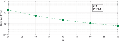
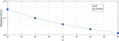
Tests for $a=2$ are shown in Figures 1 and 2, where the relative errors obtained in the comparisons of the expansions (3) and (11), respectively, to the expression given in (8) are plotted for different values of n. The calculations have been made using Matlab.

3 ALGORITHM TO COMPUTE THE ZEROS OF REVERSE GENERALIZED BESSEL POLYNOMIALS

For computing the zeros of ${\theta }_n(z;a)$ we use the results given in Reference 8. In that reference, a method for finding the complex zeros of solutions of second-order ODEs is described. The method makes use first of a qualitative analysis of the approximate Liouville-Green Stokes lines (SLs) and anti-Stokes lines (ASLs). As discussed in Reference 8, the structure of the exact zeros will follow very closely the ASLs. This qualitative analysis is combined with the application of a fixed point method $z_{n+1}=T(z_n)$ (which has fourth-order convergence and good nonlocal behavior) and the use of carefully selected step functions (displacements) $H^{\pm }(z)$.

It is important to note that the derivatives of the generalized reversed Bessel polynomials ${\theta }_n^{\prime }(z;a)$ appearing in (14) can be computed in terms of the polynomials with shifted parameters ${\theta }_{n-1}(z;a-1)$.

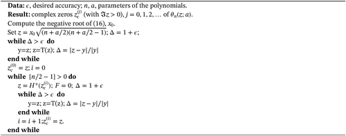
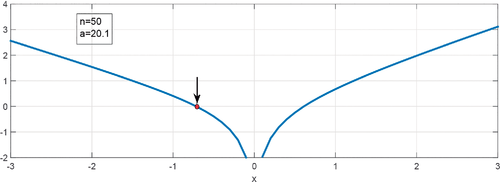
The function $g(x)$ has two real roots, one negative, $x_0$, and the other positive, $x_1$. This can be seen in the example shown in Figure 3 for a particular set of values of n and a. In our computational scheme, we will use the value $z=x_0\sqrt{(n+a/2)(n+a/2-1)}$ to iterate $T(z)$ given in (14) to obtain the first zero of the polynomials. Then, we will compute other $[n/2-1]$ zeros of ${\theta }_n(z;a)$ taking steps given by $H^{+}(z)$ and iterating each time with $T(z)$. This is summarized in Algorithm 1. This algorithm allows to compute those zeros of ${\theta }_n(z;a)$ having positive imaginary part. To complete the set of zeros of the polynomial, we just have to take the complex conjugate of each zero found (we are using the reflection formula ${\theta }_n(z;a)={\theta }_n^{\ast }(z^{\ast };a)$ for a real).

Algorithm 1. Computation of the complex zeros of ${\theta }_n(z;a)$ having positive imaginary part

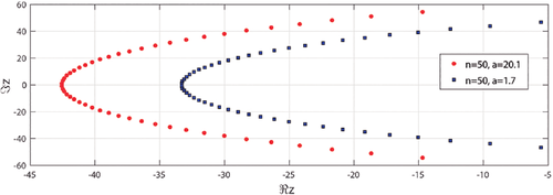
Two examples of the computation of the zeros of ${\theta }_n(z;a)$ obtained using our algorithm, are shown in Figure 4. The zeros of ${\theta }_{50}(z;a)$ evaluated for two values of a ($a=1.7,\hspace{0.17em}20.1$) are plotted in the figure. In Table 9 we give explicit values of some of the zeros found for $a=1.7$.

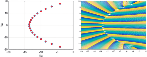
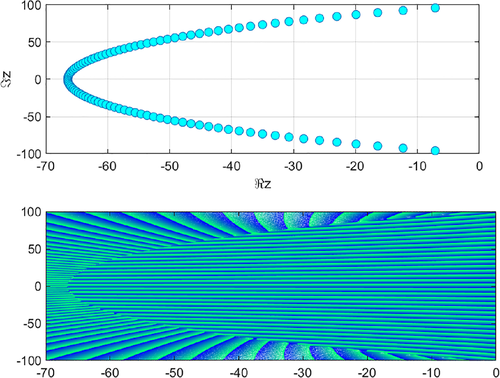
Two example of computation of the zeros for Bessel polynomials ($a=2$) are shown in Figures 5 and 6. The values of n have been fixed to 20 and 100, respectively. We also show contour plots of the modulus and phase of ${\theta }_{20}(z;2)$ and ${\theta }_{100}(z;2)$, where the position of the zeros is clearly shown in the figures. These plots are generated using Matlab and the relation to the modified Bessel function given in Equation (8). Also for the case of Bessel polynomials, explicit values of the zeros found with our algorithm are given in Table 10 for $n=12$. The calculations have been made in double precision accuracy. The function values at the zeros are also shown in the table.

4 CONCLUSIONS

The problems of computing the reverse generalized Bessel polynomials ${\theta }_n(z;a)$ and their zeros have been considered in this article. For computing the polynomials, the numerical performance of asymptotic expansions in terms of elementary functions given in Reference 5 has been illustrated with examples. We have shown that with very few coefficients in the expansions, an accuracy better or close to single precision can be obtained even for moderate values of n. We have also analyzed the conditioning of the linear homogeneous three-term recurrence relation satisfied by the polynomials. We have concluded that the polynomials are an asymptotically dominant solution of the recurrence relation. Therefore the forward computation of the recursion is well conditioned for large enough values of n. However, special care has to be taken when using the recurrence in the region where the zeros of ${\theta }_n(z;a)$ lie. With respect to the zeros of the polynomials, the computational performance of an efficient and accurate algorithm to evaluate the zeros has been shown in different examples. The method⁸ behind the algorithm is based on a qualitative analysis of the approximate Liouville-Green Stokes lines and anti-Stokes lines of the differential equation satisfied by the polynomials, combined with the application of a high-order fixed-point method and carefully selected step functions. The algorithm is shown to be efficient and accurate for all the parameters tested.