Proposition of a new index for projection pursuit in the multiple factor analysis
Abstract
This study proposes a new index for projection pursuit used to reduce the dimensions of groups of variables using multiple factor analysis. The main advantage with respect to other indexes is that the methodological procedure preserves the variance and covariance structures to perform singular value decomposition, when the index is used to compare groups of variables. Among other contributions, the study presents a modification in the grand tour algorithm with simulated annealing, adapting it to deal with groups of variables. The methodology used to assess the proposed index was based on Monte Carlo simulations, in several scenarios and with configurations of the following factors: degrees of correlation between the variables; and number of groups and degrees of heterogeneity among groups of variables. The proposed index was compared with thirteen indexes known in the literature. It was concluded that the proposed index was efficient in the reduction of data to use multiple factor analysis. This index is recommended for situations in which the groups exhibit low or high heterogeneity and a strong degree of correlation between the variables . In general terms, indexes are affected by the increase in the number of groups, depending on the scenarios assessed.
1 INTRODUCTION
In spaces with many dimensions, the samples become sparse and not very similar to each other. This fact becomes a problem when using dimensionality reduction methods based on singular value decomposition, such as the analysis of principal components, given that the information of the first components is diluted in the others. Therefore, it is advisable to reduce the dimensions without losing the information contained in the original dimension. In this context, the projection pursuit technique emerges after being suggested by Kruskal1 and implemented by Friedman and Tukey.2
In summary, projection pursuit searches for low-dimensional linear projections in high-dimensional data structures. To that end, a projection index is understood as an objective function that quantifies the degree of “interest” of a projection on the plane by vectors (orthogonal) u and v. A numerical optimization procedure is used to find the plane that maximizes this index. The problem consists in choosing the index that best represents the degree of “interest” of the projection.
It is noteworthy that projection pursuit has been implemented in several applications, namely: supervised exploratory data classification,3 robust principal component analysis,4 and independent component analysis.5 Regarding multiple factor analysis (MFA), there are no reports in the literature about the feasibility of applying this projection, or propositions of new indexes that require less computational effort with promising results.
When dealing with multiple factors analysis technique in groups of quantitative variables in high-dimensional, when applying the singular values decomposition on data in order to find the eigenvalues and eigenvectors, losses in the components explanations usually occur, by diluting the explanations on the large number of components found.
In this study, it sought to solve this deficiency, by reducing data dimensions, preserving the variances and covariance structure, to perform the decomposition, thereby ensuring a greater explanation in the first components, giving greater reliability when applying the multiple factor analysis in quantitative data in high-dimensional.
The present study proposes a new index to be used in projection pursuit applied in MFA considering groups of quantitative variables. This way, the article is divided into the following sections: Section 2—Projection pursuit and projection indexes; Section 3—Methods; Section 4—Results and discussions; Section 5—Application example; Section 6—Conclusions; and Appendix.
2 PROJECTION PURSUIT AND PROJECTION INDEX
The understanding of projection pursuit begins with a set of multivariate observations given by , each component being defined by , for i = 1, … , p. Mathematically, the projection pursuit method seeks a linear transformation, , with d < p, and T = XA, with Ap × d. This way, T is the linear projection of Xn × p, and A is the projection matrix, with the columns representing the bases of the projection space.
We are looking for linear projections with orthonormality constraints in the projection bases, that is, A · AT = In, with In being the identity matrix. This constraint ensures that each dimension of the projection space has different aspects of the data.6-8
According to Cook et al.,9 it is common to use spherical data before starting the projection pursuit, which are obtained using Equation (2), removing the influence of location and the scale for the search of structured projections. This procedure is necessary for indexes that measure the output of projected data density from a standard normal density, due to the fact that the differences in location and scale may dominate the other structural differences.
2.1 Notation
- zi is the ith observation of the spherical data of the data matrix Xn × p.
- and are n-dimensional orthonormal vectors of the projection plane.
- are the spherical observations projected on vectors and ,
Most low-dimensional projections are approximately normal.6, 11 The main appropriate indexes for reduction in dimension d ≥ 1, are described in Tables A1 and A2 (Appendix A).
The optimization of the equation is done by numerical methods, which are traditionally based on the gradient,6, 7 or the Newton-Raphson method;2, 12 however, they are not appropriate for scenarios above three dimensions.8
Other global optimizers have been proposed, for example: TRIVES,13 random scanning algorithm,14 simulated annealing,3 genetic algorithm,15 and particle swarm optimization.16
3 METHODS
In accordance with the proposed objectives of the present study, the methodology used consisted of the following steps: (i) Generation of the samples for the application of MFA (Section 3.1); and (ii) proposed index for use with MFA (Section 3.2).
3.1 Generation of samples for the application of multiple factor analysis
In order to assess the performance of the index proposed in Section 3.2, we considered several scenarios that exhibited different degrees of correlation between the variables belonging to each group, and heterogeneity between the groups. To that end, we performed the procedure proposed by Cirillo et al.,17 in which the samples were generated from normal dependent and heterogeneous populations.

The covariances represented in (6) are non-zero, since each element on the diagonal represents the jth covariance matrix of the group of variables indexed by j = 1, … , k.
- A sample of the multivariate normal distribution is simulated and a matrix Yn × pk, is obtained (Table 1). Each block of p columns (variables) corresponds to the jth group. In this way, the multivariate sampling unit is arranged in n lines.
- The observations were not altered in group 1a . The p variables of the jth group were multiplied by , defined by
()being the degree of heterogeneity among the covariance matrices specified. After completing this procedure, was adopted as parameter of the global covariance matrix defined by()with Q being a projection matrix.
| Groups | ||||||||||
|---|---|---|---|---|---|---|---|---|---|---|
| 1 | 2 | j | k | |||||||
| 1 | y111 | … | y1p1 | y112 | … | y1p2 | … | y11k | … | y1pk |
| 2 | y211 | … | y2p1 | y212 | … | y2p2 | … | y21k | … | y2pk |
| ⋮ | ⋮ | ⋱ | ⋮ | ⋮ | ⋱ | ⋮ | ⋮ | ⋮ | ⋱ | ⋮ |
| n | yn11 | … | ynp1 | yn12 | … | ynp2 | … | yn1k | … | ynpk |
| Heterogeneity among covariance matrices | Number of groups | Degree of correlation between variables |
|---|---|---|
| 2 | 7 | 0.2 |
| 0.5 | ||
| 10 | 0.9 | |
| 8 | 7 | 0.2 |
| 0.5 | ||
| 10 | 0.9 |
3.2 Proposed index for use with MFA
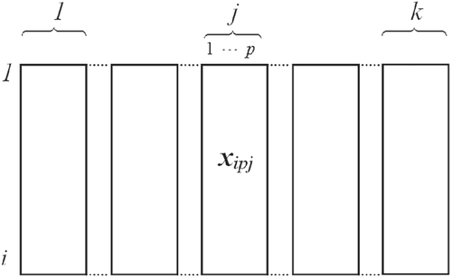
The multivariate sample was composed of groups of variables k in n observations in each group, with m = pk. This way, the observation xipj being i = 1, … , n and j = 1, … , k is identified as the ith observation in the jth group to which the pth variable belongs, as suggested by the layout of Figure 1.
It is worth noting that the equality in (10) is due to the comparison of the results with different dimensions. For example, considering matrices Xn × m and , when applying the MFA technique, we will obtain the respective eigenvector matrices V and . The similarities between the groups are expressed in Tables 3 and 4, respectively.
| Comp. | Group 1 | … | Group j | … | Group k |
|---|---|---|---|---|---|
| 1 | … | … | … | ||
| 2 | … | … | … | ||
| ⋮ | ⋮ | ⋮ | ⋮ | ⋮ | ⋮ |
| r | … | … | … |
| Comp. | Group 1 | … | Group j | … | Group k |
|---|---|---|---|---|---|
| 1 | … | … | … | ||
| 2 | … | … | … | ||
| ⋮ | ⋮ | ⋮ | ⋮ | ⋮ | ⋮ |
| … | … | … |
- Considering Xn × m a matrix of rank r by the decomposition of the singular value , and representing the square of each element in X, we have:
()with , and being the square of the elements of U, e VT, respectively (Appendix B).
- Matrix Xn × m is composed of k groups of variables, each group consisting of s > 1 variables, then we have , with xnsj representing the nth observation in the sth column of the jth group, with m = s × k. With representing the square of each element of matrix X, then, for each group j in X we have:
()with being the square of the elements of , and the square of the elements of the projections of the jth group of X in VT.
The numerical optimization to find a plane that maximized the index (16) was obtained by a modification in the grand tour algorithm (Section 3.3) using the simulated annealing method proposed by Cook et al.,19 so that groups of variables could be considered in line with the MFA.
The validation of the proposed index (16) was performed by comparing the degree of agreement in validating the reduction of projection pursuit in two dimensions for each group of variables. For this purpose, we performed 1,000 Monte Carlo simulations. Scripts were developed using the R software20 and a grand tour alternated with a simulated annealing optimization adapted for MFA (Section 3.3), with the specifications of 5e3 iteractions, cooling =0.95, eps = 1e−4, and half =30 to compute the indexes mentioned in Section 2, according to the scenarios described in Table 2 and using non-spherical data in the simulations with reduction of two dimensions in the data of each group.
3.3 Projection pursuit algorithm for the MFA technique
Input: matrix with k groups of variables.
p: number of variables in the group j.
n: number of observations.
Maxiter: maximum number of iterations.
Cooling: initial value of the cooling parameter in the range
Half: number of steps without changing Cooling.
Eps: approximation accuracy for Cooling.
for j = 1 : k do
Generate random initial projection Aa, with d < p
Perform linear transformation for the jth group.
Calculate the search index of the initial projection,
Perform h = 0, Cooling = 0.95, Half = 30, Eps = 1e−4 and i = 1.
while(i < Maxiter and Cooling > Eps) do
Generate a new random projection Ai.
Then, generate a new projection .
Perform , interpolation from the projection Aa
until projection .
Perform linear transformation , for jth group.
Calculate .
if do
Perform Aa = Az,
else
Perform h + =1
end if
if h = Half then
Perform and h = 0
end if
Perform i + =1
end while
Perform , which represents the matrix with the reduced dimension
of the jth group
end for
The new matrix with k groups of variables with reduced dimensions will be
represented by:
Output: The MFA technique is applied to groups formed in .
4 RESULTS AND DISCUSSIONS
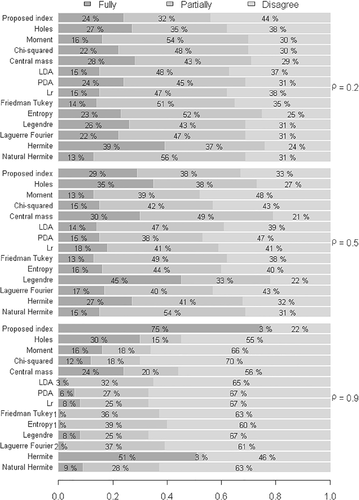
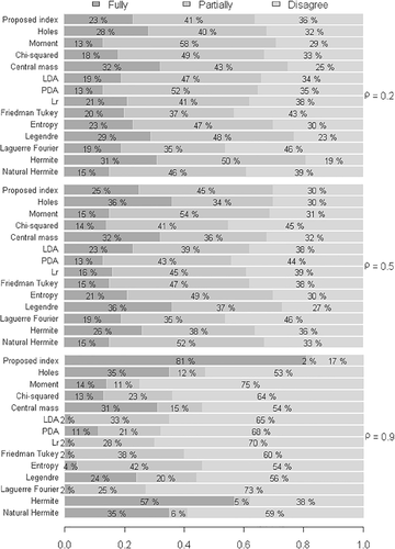
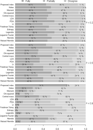
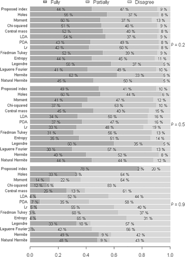
According to the proposed objectives of the present study, the results shown in Figures 2-5 correspond to the reduced dimensions relating to the first principal component, precisely because it always presents the greatest explanation in MFA. This way, the results were presented as follows: (i) Evaluation of the proposed index with respect to the heterogeneity between the groups (Section 4.1); and (ii) evaluation of the proposed index with respect to the increase in the number of groups (Section 4.2).
4.1 Evaluation of the proposed index with respect to the heterogeneity between the groups
The results illustrated in Figure 2 indicate that the proposed index initially exhibited a high discordance rate in comparison to the other indexes, when considering a weak degree of correlation between the variables . However, as the degree of correlation increased, this rate was reduced. This way, maintaining a strong degree of correlation between the variables , the proposed index resulted in low disagreement and promising results with respect to agreement with the others. It is worth noting that the simulated data were non-spherical, a condition that usually undermines the applicability of the proposed indexes.
In view of the above, in order to compare the validation of the index for the same scenarios, even though the degree of heterogeneity between the groups was increased , the results illustrated in Figure 3 were compared with the condition of low heterogeneity illustrated in Figure 2.
The results illustrated in Figure 3 practically confirmed the same behavior of the indexes with respect to the degree of correlation between the variables and the degrees of agreement and disagreement between the indexes. Virtually, any difference results from error oscillation in the Monte Carlo method. However, a result that should be highlighted was the strong degree of correlation . In this context, we observed that the proposed index exhibited a high degree of agreement when the samples were simulated for a low degree of heterogeneity , with a percentage close to 75%. When the index was increased to , it exhibited considerable improvement, with a percentage of agreement close to 81%.
4.2 Evaluation of the proposed index with respect to the increase in the number of groups
Compared with the results illustrated in Figure 2, in which low heterogeneity was considered between groups and groups , it is noted in Figure 4 that, with the same configurations, the increase in the number of groups confirmed that the degrees of agreement and disagreement of the proposed index were approximately equal when . Therefore, there is statistical evidence that the index yields promising results when the variables are strongly correlated, regardless of the dimension of the group.
Considering the high heterogeneity between the groups , the increase in the number of groups , in general terms, did not affect the performance of the indexes. Figure 5 shows that the same behavior of the indexes occurred regarding the degree of correlation and the agreement rate in comparison with the competing indexes.
It should be emphasized that in all simulated scenarios, in conditions of poor and moderate correlation the proposed index exhibited a reduction in the disagreement rate with respect to its competitors. In this context, there is evidence to affirm that, on average, all indexes are affected by the increase in the number of groups. This way, it can be affirmed that the occurrence of these results does not prevent the application of the indexes evaluated in the present study, that is, projection pursuit applied in MFA.
5 EXAMPLE OF APPLICATION
For the didactic purpose, this section contains an example of the use of MFA, and an example of the use of MFA with dimension reduction using projection pursuit with the proposed index.
5.1 Use of the MFA technique
We simulated three groups of variables (Table 5). The data of each group were generated according to the methodology described in Section 3.1, using the parameters and .
| Group 1 | Group 2 | Group 3 | ||||||||
|---|---|---|---|---|---|---|---|---|---|---|
| Obs. | V1 | V2 | V3 | V4 | V5 | V6 | V7 | V8 | V9 | V10 |
| 1 | 1.39 | 2.44 | 3.06 | 4.35 | 1.75 | 2.13 | 2.88 | 1.90 | 3.08 | 3.58 |
| 2 | 0.98 | 1.85 | 3.02 | 3.76 | −0.42 | 0.19 | 1.38 | 1.58 | 2.05 | 3.76 |
| 3 | 2.38 | 3.56 | 4.37 | 5.40 | 0.03 | 1.27 | 1.76 | −0.06 | 1.21 | 2.21 |
| 4 | 1.51 | 2.41 | 3.68 | 5.31 | 0.33 | 1.02 | 2.36 | 0.62 | 2.40 | 3.58 |
| 5 | 0.53 | 1.69 | 1.88 | 4.24 | 1.01 | 2.41 | 2.41 | 1.73 | 3.10 | 3.66 |
| 6 | 1.40 | 2.02 | 3.40 | 3.58 | 1.03 | 2.56 | 3.16 | 1.24 | 1.89 | 2.77 |
The explanations of the principal components described in Table 6 were obtained applying the MFA technique,18 with scripts elaborated using the R software and the MVar package.21
| Components | Eigenvalues | % of variance | % accumulated variance |
|---|---|---|---|
| 1 | 2.0010 | 57.79 | 57.79 |
| 2 | 0.9087 | 26.24 | 84.03 |
| 3 | 0.3335 | 9.63 | 93.66 |
| 4 | 0.1294 | 3.74 | 97.39 |
| 5 | 0.0902 | 2.61 | 100.00 |
The inertia of the groups of variables are described in Table 7.
| Group | Comp. 1 | Comp. 2 | Comp. 3 | Comp. 4 | Comp. 5 |
|---|---|---|---|---|---|
| 1 | 0.8240 | 0.0915 | 0.1803 | 0.0626 | 0.0298 |
| 2 | 0.3052 | 0.6991 | 0.0191 | 0.0407 | 0.0340 |
| 3 | 0.8718 | 0.1181 | 0.1341 | 0.0260 | 0.0264 |
| 2.0010 | 0.9087 | 0.3335 | 0.1294 | 0.0902 |
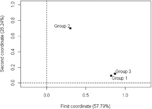
With respect to the first principal component, Table 7 shows that groups 1 and 3 exhibited strong similarity between them (0.8240 and 0.8718, respectively) and group 2 differed from the others. Regarding the second component, it can be affirmed that groups 1 and 3 were similarly weak, and group 2 remained original. Other analyzes could have been performed with the other components; however, as full explanation had already been given by the first component—with the greatest explanation (57.79%)—no other explanation was necessary besides that given by the first principal component.
From the inertias obtained in the groups (Table 7), aiming at a better interpretation, a chart of inertia (Figure 6) was elaborated showing that there was strong relationship between groups 1 and 3 with respect to the first component, thus confirming the originality of group 2.
5.2 Use of the MFA technique with dimension reduction performing projection pursuit with the proposed index
We used matrix X6 × 10 illustrated in Table 5 of Section 5.1. We obtained the projection matrices for each group with the projection indexes (Table 8) by applying projection pursuit with the proposed new index presented by Equation (16), and new algorithm presented in Section 3.3.
| Group 1 | Group 2 | Group 3 | ||||
|---|---|---|---|---|---|---|
| Projection | Vector 1 | Vector 2 | Vector 1 | Vector 2 | Vector 1 | Vector 2 |
| 1 | −0.2438 | 0.9151 | −0.7770 | −0.0341 | 0.5207 | 0.3659 |
| 2 | 0.6822 | 0.0018 | −0.5748 | −0.3685 | −0.0633 | 0.9175 |
| 3 | 0.6545 | 0.2296 | 0.2565 | −0.9289 | 0.8513 | −0.1555 |
| 4 | 0.2160 | 0.3312 | − | − | − | − |
| Projection index | 0.16686 | 0.17255 | 0.17860 | |||
Figure 7 shows the convergence of the new index for each group of variables in the numerical optimizations.
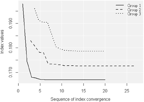
When we applied the projection matrices in the groups in X6 × 10, we obtained the data shown in Table 9, which represent the data with reduced dimensions in two dimensions for each set Xj, so that matrix X6 × 10 will be represented by the new matrix .
| Group 1 | Group 2 | Group 3 | ||||
|---|---|---|---|---|---|---|
| Obs. | Projection | Projection | Projection | Projection | Projection | Projection |
| 1 | 2 | 1 | 2 | 1 | 2 | |
| 1 | 4.2683 | 3.4201 | −1.8451 | −3.5201 | 3.8420 | 2.9645 |
| 2 | 3.8121 | 2.8392 | 0.5712 | −1.3376 | 3.8939 | 1.8744 |
| 3 | 5.8753 | 4.9768 | −0.3017 | −2.1040 | 1.7735 | 0.7445 |
| 4 | 4.8318 | 3.9902 | −0.2371 | −2.5795 | 3.2185 | 1.8722 |
| 5 | 3.1702 | 2.3242 | −1.5517 | −3.1615 | 3.8203 | 2.9082 |
| 6 | 4.0356 | 3.2515 | −1.4610 | −3.9142 | 2.8841 | 1.7571 |
We applied the MFA technique in the new groups of variables (Table 9). The explanations of the principal components are given in Table 10.
| Components | Eigenvalues | % of variance | % accumulated variance |
|---|---|---|---|
| 1 | 2.0306 | 65.33 | 65.33 |
| 2 | 0.8681 | 27.93 | 93.26 |
| 3 | 0.1678 | 5.40 | 98.66 |
| 4 | 0.0382 | 1.23 | 99.89 |
| 5 | 0.0034 | 0.11 | 100.00 |
The inertias of groups of variables with reduced dimensions are described in Table 11.
| Group | Comp. 1 | Comp. 2 | Comp. 3 | Comp. 4 | Comp. 5 |
|---|---|---|---|---|---|
| 1 | 0.8278 | 0.0956 | 0.0768 | 0.0009 | 0.0001 |
| 2 | 0.3300 | 0.6705 | 0.0065 | 0.0273 | 0.0010 |
| 3 | 0.8727 | 0.1021 | 0.0846 | 0.0100 | 0.0023 |
| 2.0306 | 0.8681 | 0.1678 | 0.0382 | 0.0034 |
The same observations made in Table 7, which deal with the similarities of groups of variables with original dimensions, apply to Table 11. Regarding the first principal component, groups 1 and 3 exhibited strong similarity between them, and group 2 differed from the others.
Aiming at a better interpretation, the chart of inertia illustrated in Figure 8 was again elaborated from the inertias of the groups shown in Table 11. There was strong relationship between groups 1 and 3, again confirming the originality of group 2.
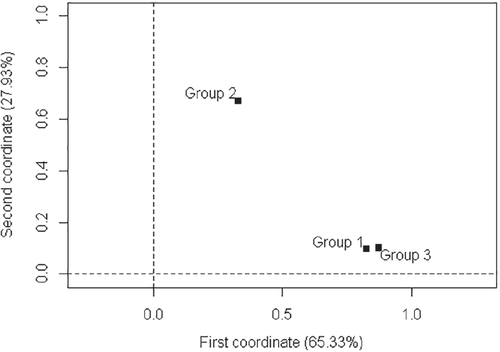
As can be observed, the results of the similarities in data with reduced dimensions produced the same results than the data with original dimensions. This fact demonstrates the efficiency of the proposed new index with application in MFA using high-dimensional data.
6 CONCLUSIONS
The proposed new index proved to be efficient in the reduction of data for application in the MFA technique. This index is recommended for situations in which the groups exhibit low or high heterogeneity, and a strong degree of correlation between the variables . In general terms, indexes are affected by the increase in the number of groups according to the scenarios evaluated.
APPENDIX A: TABLES
| Index (PI) | Characteristics |
|---|---|
| Holes22 | Obtained by means of the normal density function, being sensitive to projections with few points in the center. |
| Central mass22 | Obtained by means of the normal density function, being sensitive to projections with many points in the center. |
| LDA8 | Obtained through linear discriminant analysis in order to find linear projections with the greatest separation between classes and the lowest intra-class dispersion. |
| PDA23 | Penalized discriminant analysis, it is based on penalized LDA, being applied in situations with many highly correlated predictors when classification is required. |
| Lr-norm3 | It is based on the supervised exploratory classification, being used in the detection of outliers. |
| Index (PI) | Characteristics |
|---|---|
| Moments10 | It is based on the third and fourth bivariate moments, being used mainly in large datasets. |
| Chi-square24 | Based on the chi-square distance, considering certain divisions in the projection plane, and the radial symmetry of the normal bivariate distribution. |
| Friedman-Tukey2 | It is based on interpoint distances in the search for optimum projection. The directions chosen are those that maximize the coefficient, providing the greatest separation for the different clusters. By means of a recursive process, the index is applied again to each cluster in order to find new projections that reveal more clusters. |
| Entropy7 | It is an extension of the Friedman-Tukey index constructed using the negative entropy of a density core estimate. |
| Legendre25 | Based on distance L2 between the density of the projected data and the standard normal bivariate density. It is constructed by inversion of density through a normal cumulative distribution function with the transformations and , where is the standard normal distribution, and using J terms of Legendre polynomials for expansion. |
| Laguerre-Fourier25 | Based on distance L2 between the projected data density and the standard normal bivariate density in polar coordinates, with and , and using K terms of a Fourier series and the radial part in L terms of Laguerre polynomials. |
| Hermite10 | Based on distance L2 between the density of the projected data and the standard normal bivariate density. Expanding the function - marginal density of Z in plane - in H terms of Hermite polynomials being orthogonal to (standard normal distribution). |
| Natural Hermite10 | Based on distance L2 between the density of the projected data and the standard normal bivariate density. Expanding the function in N terms of Natural Hermite index being orthogonal to (standard normal bivariate distribution). |
APPENDIX B: R CODE EXEMPLIFICATION OF SOME MATRIX RESULTS
-
n <- 10
-
p <- 3
-
X <- matrix(rnorm(n*p), nrow = n)
-
X <- round(cbind(X, X[, 1:2] + matrix(rnorm(20) * 0.000001, nrow = n)), 3)
-
svd.x <- svd(X)
-
U <- svd.x$u[, 1:3]
-
L <- svd.x$d[1:3]
-
V <- svd.x$v[, 1:3]
-
U %*% diag(L) %*% t(V)
-
sum(X∧2)
-
sum(U∧2 %*% diag(L∧2) %*% t(V∧2))
Biographies

Paulo César Ossani PhD holder in Statistics and Agricultural Experimentation (Universidade Federal de Lavras/UFLA, 2019) and PostDoc at Universidade Federal de Maringá (UEM, 2020). Working with Multivariate Statistics, Computational Statistics, Machine Learning and software development to aid in the solving of mathematical and statistical problems.

Mariana Figueira Ramos graduate in Statistics (Universidade Federal do Espirito Santo, 2010) and Master's degree in Statistics and Agricultural Experimentation (Universidade Federal de Lavras, 2013). Working with digital business. Seasoned in the field of Probability and Statistics with focus in classification. Working specially with the following topics: multivariate analysis, discriminant analysis, logistic regression, and correspondence analysis.

Marcelo Ângelo Cirillo Associate Professor at Universidade Federal de Lavras, Department of Exact Sciences, working with graduate researches and tutoring in the following fields: Multivariate Analysis, Computational Statistics, Generalized Models and Response Surface Methodology. All the statistical methodologies are applied in agrarian sciences and food sciences.


