Diaphysator: An online application for the exhaustive cartography and user-friendly statistical analysis of long bone diaphyses
Funding information: Grantová Agentura, Univerzita Karlova, Grant/Award Number: GAUK no. 250 057; STARS (Supporting TAlented PhD Research Students, Charles University)
Abstract
The cross-sectional geometry (CSG) of long bone diaphyses is used in bioanthropology to evaluate their resistance to biomechanical constraints and to infer life-history-related patterns such as mobility, activity specialization or intensity, sexual dimorphism, body mass and proportions. First limited by technical analytical constraints to the analysis of one or two cross sections per bone, it has evolved into the analysis of cross sections of the full length of the diaphyseal part of long bones. More recently, researchers have developed analytical tools to map the cortical thickness of entire diaphyses to evaluate locomotor signatures. However, none of these analytical tools are easy to use for scientists who are not familiar with computer programming, and some statistical procedures–such as mapping the correlation coefficients of the diaphyseal thickness with various parameters have yet to be made available. Therefore, we developed an automated and open-source application that renders those analyses (both CSG and cortical thickness) in a semiautomated and user friendly manner. This application, called “Diaphysator”, is associated with another free software (“Extractor”, presented in Dupej et al. (2017). American Journal of Physical Anthropology, 164, 868–876). Diaphysator can be used as an online application (https://diaphysator.shinyapps.io/maps) or as a package for R statistical software. Along with the mean maps of cortical thickness and mean CSG parameter graphs, the users can evaluate the correlations and partial correlations of both CSG parameters at every cross section along the diaphyseal length, and cortical thickness data points of the entire diaphysis, with any factor such as age, sex, stature, and body mass.
1 INTRODUCTION
The study of bone biomechanics in biological anthropology has spread following the analyses developed by Ruff and Hayes (1983a, 1983b). Those analyses are based on the premise that bone is a living tissue that functionally adapts to changes in its mechanical environment by remodeling accordingly. The efficiency of the remodeling (or of the modeling when it occurs prior to the end of the skeletal maturation) varies with age (e.g., Doyle, Lazenby, & Pfeiffer, 2011; Ruff & Hayes, 1984; Šešelj et al., 2012). Sex specificities have been found (Beck et al., 1992; Ruff, 1987; Ruff & Hayes, 1983b; Ruff & Hayes, 1988), and the related study of hormonal influence is still a growing field (Heaney et al., 1997; Petit et al., 2004; Van Caenegem et al., 2012). The functional adaptation also differs by bone (Schlecht, Bigelow, & Jepsen, 2014) and between skeletal sites of a single bone (Ruff, Scott, & Liu, 1991). Specifically, the diaphyseal part of long bones is composed of cortical bone, a dense and compact material, that makes it more labile to biomechanical variations than its porous counterpart, which is found mostly in the articulations and is composed of a network of intricate trabeculae (Ruff, 1988, 2002).
To infer life history from the skeleton, the diaphyseal part of long bones is therefore an ideal potential tool. Using engineering models applied to bone shafts (known as the study of cross-sectional geometry or CSG), researchers could estimate bone resistance to various mechanical constraints (and their direction) to understand the cause of variations in diaphyseal geometry (Ruff & Hayes, 1983a, 1983b). Thus, the discipline known as cross-sectional geometry advanced greatly and could test almost as many hypotheses as there are variations in bone shape: senescence, sexual dimorphism, sexual division of labor, intensity and repetitiveness of activities, specialized activities, locomotion, body mass, body proportions and size (e.g., Martin & Atkinson, 1977; Ruff, 1987; Ruff et al., 1991; Shaw & Stock, 2009a, 2009b; Trinkaus, Churchill, & Ruff, 1994). In the first years, the method required cutting the bones to measure them, which did not allow for the analysis of more than one or a few cross section(s) per bone (Ruff & Hayes, 1983a, 1983b). However, the variation of a single bone across skeletal sites in terms of thickness, size of the areas or other geometry parameters, as considered from the cross sections, was always known, although it was not possible to always consider the diaphysis as a whole (Ruff, 1987).
Because CT scanning techniques became more accessible, measuring diaphyseal bone became a virtual operation. Therefore, some researchers started developing methods to map the cortical thickness and automatize the measurement of areas on dozens of cross sections of entire diaphyses (Doube et al., 2010; Puymerail et al., 2012, b; Ruff, Puymerail, Macchiarelli, Sipla, & Ciochon, 2015; Zanolli, Bayle, & Macchiarelli, 2010). The maps have been first used to identify the functional signature of postural and locomotor patterns that impact the diaphyseal shape of lower limb long bones (Puymerail, Ruff, et al., 2012; Puymerail, Volpato, et al., 2012; Ruff et al., 2015; Zanolli et al., 2010). Those methods are still being improved to date (Bondioli et al., 2010; Doube, Conroy, Christiansen, Hutchinson, & Shefelbine, 2009; Dupej, Lacoste Jeanson, Pelikán, & Brůžek, 2017; Morimoto, Zollikofer, & Ponce de León, 2012). After improving the mapping techniques using tools inherited from morphometric analysis to render the diaphyseal thickness maps more homologously (Dupej et al., 2017), procedures have been developed to map the correlations between diaphyseal thickness and body covariates (Lacoste Jeanson, Santos, Dupej, Velemínská, & Brůžek, 2018; Lacoste Jeanson, Santos, Villa, Banner, & Brůžek, 2018). Finally, inspired by the work developed by experts in dental topography (Guy, Gouvard, Boistel, Euriat, & Lazzari, 2013; Le Luyer, Rottier, & Bayle, 2014), graphical representations of the long bone architecture at every cross section along the diaphysis were automatically built (Lacoste Jeanson, Santos, Dupej, et al., 2018; Lacoste Jeanson, Santos, Villa, et al., 2018). However, some of the analytical tools to study the entire diaphysis and perform statistical analysis with them have yet to be released. To fill this gap, this article intends to present an open source, cross-platform and user-friendly application designed to semiautomatically build cartographies of thickness and correlations of entire diaphyses, as captured by CT scans.
2 A FULL ECOSYSTEM
2.1 Extractor
Diaphysator functions in symbiosis with the software Extractor published in 2017 (Dupej et al., 2017). As input files, Diaphysator requires the data files to be generated by the Extractor or text files to be manually created and formatted in the same way. The webpage containing the application also hosts the Extractor, but the latter functions offline and exclusively in a Windows environment.
The Extractor is a semiautomatic workflow developed to analyze long bone full diaphysis. Based on three specific landmarks provided by the user, it automatically extracts both endosteal and periosteal surfaces of the diaphysis directly from CT scans converted into the RAW format. The software minimizes the potential error or variation induced by manual landmark placing by performing landmark refinement using rigid registration (rotation, translation, and scaling). This procedure ensures the homology between the extracted data, which is paramount for further statistical analysis of the data. Because the Extractor reslices the diaphyses into virtual cross sections along the medial axis and is based on an adaptive thresholding method for boundary detection called the half-maximum height (Spoor, Zonneveld, & Macho, 1993), it automatically extracts diaphyseal data and make them homologous, even from CT scans of living individuals (containing soft tissues) who have not been specifically positioned prior to being scanned. The Extractor also evaluates the radius of the medial axis, namely, the inner curvature.
2.2 Diaphysator
Diaphysator is essentially a tool for data visualization and simple statistical processing for the files produced by the Extractor. Particularly, Diaphysator cannot handle mesh files and is dedicated to the analysis of raw Comma-separated values (CSV) files, such as those obtained by the Extractor. It includes several features to generate maps based on cortical thickness maps (by default, n = 5,000 data points/diaphysis) and graphs based on cross-sectional geometry measured on multiple cross sections along the diaphysis (by default, n = 100 cross sections/diaphysis). From those maps and graphs, Diaphysator automatically allows comparisons between groups of individuals and calculates correlation coefficients of the maps and graphs with a given covariate. The application can also calculate partial correlation coefficients to control for the effect of one covariate on a pair of other variables.
Diaphysator can be used either as an online application (https://diaphysator.shinyapps.io/maps), thus requiring no other software than a web browser, or as a package for the R statistical software (R Core Team, 2018) hosted on a GitLab repository (https://gitlab.com/f.santos/Diaphysator). Detailed instructions for installing and using Diaphysator, along with written and video tutorials and all the data files used in this article, can be found at: http://projets.pacea.u-bordeaux.fr/logiciel/extractor/extractor_diaphysator.html. This R package will be maintained by one of the authors (FS) and is likely to evolve regularly.
The graphical user interface was coded using the R package shiny (Chang, Cheng, Allaire, Xie, & McPherson, 2018), which allows the construction of user-friendly, interactive, and reactive web pages; this allows statistical analysis to be entirely performed through an Internet browser window, without requiring any knowledge of the R language. R-Shiny applications are particularly useful for scientists who are not familiar with computer programming, and such applications are becoming increasingly popular in various subfields of biological anthropology (Berg & Kenyhercz, 2017; Gonçalves et al., 2016; Lynch, 2018; Santos, 2018).
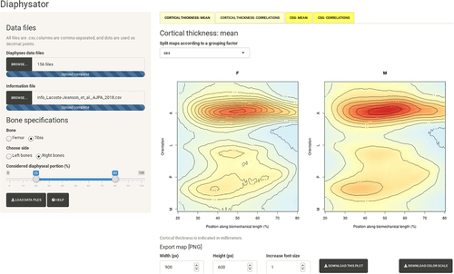
An overview of the graphical user interface of Diaphysator is given in Figure 1. In the left panel, the user is invited to provide the input data files from two different sources. First, the multiple CSV files (each containing the diaphyseal data for a given individual) generated by the Extractor can be loaded at once. Second, a separate CSV file (hereafter referred to as “information file”), which must be manually created upstream, must be imported to provide additional details about the individuals, such as age, sex, country, body composition variables (fat mass, fat-free mass), and stature. These variables, which can be freely determined and named by the user, are then available in the user interface of Diaphysator to be correlated with the data extracted from CT scans. Still in the left panel, the user needs to specify which bone (femur or tibia) and which side (left or right) are considered, and which portion of the diaphysis has been extracted–this value is by default between 20% (located in the distal part of the diaphysis) and 80% (proximally) of the selected total bone length. Although this portion is selected by default because it is also the default setting for the Extractor, the user can specify here the portion of the considered bone length that corresponds to the data input files.
3 INTRODUCING DIAPHYSATOR
3.1 Cortical thickness
Cortical thickness is the distance between the periosteal and endosteal surfaces of the long bone shaft. Using the extractor, the cortical thickness is, by default, computed for the portion between 20% (distal) and 80% (proximal) of the biomechanical length (defined as the distance between the two landmarks located at each extremity of the long bone and that the user supplied the Extractor with). In case values other than the default ones have been used, the user must specify which values were used in the left panel of the user interface of Diaphysator before importing the data.
By default, with the extractor, 100 cross-sections are considered within this diaphyseal segment, and thickness is measured in 50 directions (which correspond to equally spaced angular increments from the cross-section centroid) per cross section, bringing the total number of data points that describe the diaphyseal thickness (i.e., the distance between the endosteal and periosteal surfaces) to 5,000 per diaphysis. Custom values for the number of slices and directions can be used with the Extractor and are automatically detected by Diaphysator by inspecting the dimensions of the data input files.
With the Extractor, cortical thickness is calculated for each point of the periosteal surface as the distance to the closest point of the endosteal surface. Our approach does not simplify the medial axis to a straight line, instead the Extractor detects the centroids of each slice containing diaphyseal bone. Bone boundary is identified with an adaptive thresholding method, called half-maximum height (Spoor et al., 1993) as implemented by Dutailly, Coqueugniot, Desbarats, Gueorguieva, and Synave (2009).
The first tab of results of Diaphysator returns a map of the average cortical thickness along the extracted portion of the diaphysis. A separate map can be obtained for each level of a grouping factor (such as sex or age categories) provided in the information file. Like any other graph displayed in Diaphysator, this map, along with its color scale, can be downloaded in the PNG format through the graphical interface.
The second tab of results returns a map of the correlation between the cortical thickness and any numeric variable—such as body mass—provided in the information file, thus allowing for the identification of bone areas that covary the most or least with this variable. The correlation can be assessed with any of the three usual correlation coefficient formulae (Pearson, Kendall, or Spearman). Partial correlations are also available, allowing a third control variable to also be retrieved from the information file.
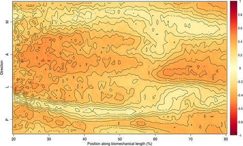
For both tabs, the vertical axis of the maps automatically indicates the posterior, medial, anterior, and lateral bone surfaces of the bone. When the cortical data uploaded in Diaphysator corresponds to a set of femora, the posterior face is determined as the direction at which the average cortical thickness is maximal along the portion of the diaphysis (matching the linea aspera), and the other faces are placed accordingly, given the lateralization (left or right) specified by the user. If the bones are tibiae, the location of the maximal thickness corresponds to the anterior face, and the other faces are placed accordingly.
3.2 Cross-sectional geometry
CSG provides an estimation of the resistance of the diaphysis to various directional and mechanical constraints as if it was a beam. It is based on formulae developed from the dimensions and areas of single cross sections taken along a long bone diaphysis. By default, the Extractor computes the medullary area (MA) and total area (TA) of 100 cross sections contained within the portion located between 20% and 80% of the biomechanical length. From those, Diaphysator automatically calculates the cortical area (CA) and relative proportion of CA within the total area of the cross section (CA%). Areas of the cross sections are considered to be proportional to compressive and tensile forces and should therefore be a good proxy to estimate bone axial strength if the bone was not curved (Ruff, 1989; Ruff & Hayes, 1983a).
The last two tabs of results of Diaphysator display the following: the averaged cortical areas of the selected number of cross sections along a specific portion of the diaphysis, and the curves of the absolute correlation coefficients of cortical or medullary areas measured on diaphyseal cross sections with any numeric covariate that is selected from the information file. These results can still be obtained for each level of a grouping factor such as sex or age categories, and the options detailed in the previous section for the calculation of correlation coefficients remain available.
4 CASE STUDY
To test the efficiency of both the Extractor and Diaphysator, we used a sample of whole-body CT scans performed on cadavers at the University of Copenhagen, Department of Forensic Medicine, Unit of Forensic Anthropology in Copenhagen, Denmark (Lacoste Jeanson, Dupej, et al., 2017; Lacoste Jeanson, Santos, et al., 2017; Villa et al., 2017). The bodies have not been positioned in a standardized fashion prior to scanning. The female sample used in this study is part of the Danish project “SURVIVE: Let the dead help the living,” a prospective, nationwide autopsy-based study carried out in collaboration with the Forensic Institutes in Copenhagen, Odense, and Aarhus. No formal ethical consent is needed from Danish ethical committees to work with CT images of dead humans. Medico-legal autopsies are mandated by the police, and CT scans are part of the routine investigation at the Department of Forensic Medicine (University of Copenhagen). The Department of Forensic Medicine adheres to Danish standards accreditation regarding data security. No personalized data can be exported from the systems. All personal data are removed from all images because they have no use in the project; only age, sex and stature were retained for this case study. The sample consists of 36 males and 42 females. Full descriptive data of the sample can be found elsewhere (Lacoste Jeanson, Dupej, et al., 2017; Lacoste Jeanson, Santos, et al., 2017; Villa et al., 2017). The full data, along with those of the tibial diaphysis, are publicly available on Zenodo (Lacoste Jeanson, 2019) or by clicking the “Help” button in the Diaphysator user interface.
From those 78 CT scans, both surfaces (endosteal and periosteal) of the right femoral diaphyses were semiautomatically extracted, which ensured homology and minimized input error by users using the Extractor (Dupej et al., 2017). The selected segment was between 20% and 80% of the total biomechanical length. From those extracted diaphyses, the Extractor evaluated the cortical thickness at 5,000 data points and measured the areas (medullary and total) of every cross section (by default, n = 100). Two sheets in the CSV format containing these measures were automatically created for each diaphysis.
We imported into Diaphysator the automatically created data files containing the area and thickness of each diaphysis. We also imported an information file containing the age, sex, and stature of the individuals.
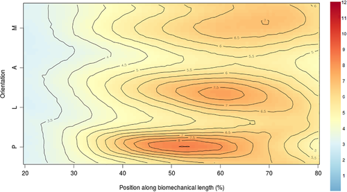
We first mapped the cortical thickness data of the femur. The mean values of thickness for the studied sample are found in Figure 2. The application could also separate the maps according to a categorical variable such as sex. The anterior, lateral, posterior, and medial surfaces of the bone are unrolled along the vertical axis. The location along the diaphysis is depicted along the horizontal axis, with 20% being the most distal point and 80% the most proximal. The thickness is graphically represented on a chromatic scale from light blue (very thin) to dark red (very thick). As explained above, the location of the maximum thickness is located on the posterior surface of the diaphysis, matching the linea aspera, where numerous muscles attach.
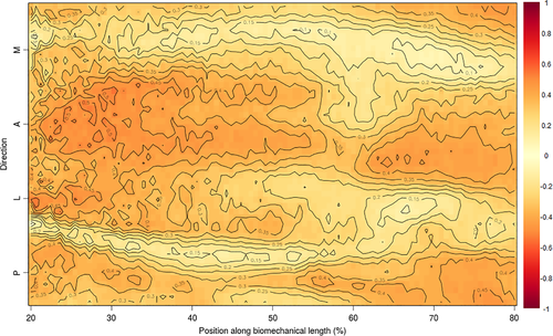
Next, we considered the correlations between cortical thickness and stature (Figure 3). Pearson correlation coefficient values (r) are represented here on a heat scale from light yellow (corresponding to a correlation coefficient close to 0) to red (corresponding to strong positive or negative correlations, |r| ≈ 1). The femoral diaphyseal thickness displays relatively high correlations with stature, especially in the distal half between the anterior and lateral surfaces (|r| > 0.5). Stature might also be a factor moderately correlated with the whole length of the posterior surface of the femoral diaphysis, with correlation coefficients reaching 0.4. The application gives the option to use partial correlations to control the effect of a selected variable on the relationships found between cortical thickness and another covariate. Here, we controlled for the effect of age on the observed relationships between stature and cortical thickness (Figure 4). The pattern of correlations does not vary much from Figure 3; the area located from 20% to 40% of the antero-lateral surfaces of the femoral biomechanical length displays correlation coefficients only slightly lower than those in Figure 3—the difference in correlation coefficient values being usually inferior to 0.05. This suggests that age does not have a decisive influence on the relationship observed between femoral cortical thickness and stature.
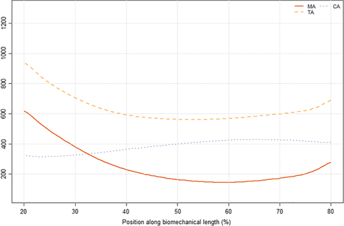
We also plotted the CSG parameters as measured on 100 slices within the portion located between 20% and 80% of the femoral biomechanical length (as depicted along the horizontal axis). The vertical axis of the automatically generated graphs represents the values of the correlation coefficients. Similar to cortical thickness, it is also possible to define whether the average value of the sample could be separated by a given categorical value. Here, we chose again to present the graphs sex-pooled (Figure 5). The total and medullary areas of both sexes show a continuous increase toward the distal end of the diaphysis, while cortical areas display more linear values along the length of the diaphysis.
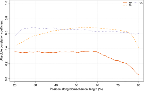
Correlation coefficients of the cortical bone areas and age have also been computed for this sample (Figure 6). The highest correlations are found with cortical areas and total areas (|r| > 0.6). Correlation coefficients according to stature diminish toward the extremities of the diaphysis for total areas, suggesting that if stature is a factor of influence in the femoral architecture, it might be less the case for the epiphyses than for diaphyses. Medullary areas display correlations lower than 0.4, indicating that their size might be shaped by another factor than purely stature.
In summary, this article presented an online application–Diaphysator–that can handle the automatic statistical processing of a large amount of data derived from the measurement of the architecture of long bone diaphyses, that is, cross sectional geometry parameters and thickness data. The application functions symbiotically with a previously released computer software–Extractor–by automatically processing files created semi-automatically from the extraction of diaphyseal data from the Extractor. Although this article presented and released a human dataset of the femur and tibia, Diaphysator could handle nonhuman species and other long bone diaphyses in a future version. This only requires that three homologous landmarks can be found on the said bones–so that they can be processed with the Extractor upstream–, and a simple rule to detect automatically the faces (posterior, medial, anterior, and lateral) can be defined.
DATA ACCESSIBILITY
The data that support the findings of this study are openly available in Zenodo at http://doi.org/10.5281/zenodo.2593489, reference number 2593489.


